Applications of Petroleum Exploration and Environmental Geochemistry to Carbon Sequestration
Robert J. Pirkle,
![]() Microseeps Inc., 220 William Pitt Way, Pittsburgh, PA 15238
Microseeps Inc., 220 William Pitt Way, Pittsburgh, PA 15238
&
Victor T. Jones,
![]() Exploration Technologies, Inc., 7755 Synott, Houston, Tx 77083
Exploration Technologies, Inc., 7755 Synott, Houston, Tx 77083
(Printable Copy - FinalVersion1.10.pdf)
ACKNOWLEDGEMENTS
The preparation of this document was supported by The Lawrence Berkeley National Laboratory under LBNL Subcontract No. 6804108. The authors wish to thank Dr. Sally M. Benson for her encouragement, support and interest in this effort. The authors would like to express their sincere appreciation to Mr. Patrick Myers for his assistance in editing the manuscript and figures, and for creating a readable and coherent electronic document.
Table of Contents
SOIL GAS ANOMALIES OVER PETROLEUM RESERVOIRS
- The Pineview Oil Field Survey
- The Pleasant Creek Gas Storage Field Survey
- The Hartzog Draw Oil Field Survey
- The Marquez Field Survey
- The Weyland Oil Field Survey
- The Kansas-Colorado State Line Complex Survey
- The Joliett Field Drop Core Survey
- The Gulf Marine Geochemical “Sniffer” Detector
- Marine Anomalies and Brightspots
- The High Island Surveys
- Pine Valley Surveys
- Snake Valley Surveys
- Wyoming Underground Coal Gasification Reactor Monitoring
- Salt Dome Cavern Monitoring
- The Barbers Hill Salt Dome Cavern Leak
- A Mississippi Salt Dome Cavern Leak
- A Mined Gas Storage Cavern Leak
- Barometric Pressure and its Relationship to Gas Flux
- Mined Gas Cavern Example
- The Savannah River Site Sanitary Landfill Example
- Western Salt Block Cavern Example
- Deep Mobile Gases and Their Relation to Earthquakes
- San Andreas Fault Example
- The Pacoima Dam Example
- Arrowhead Hot Springs Example
- The Playa Vista Example
- Vadose Zone Vertical Migration Pathways and Interferences
- Flux Pipes and Footprints
- Effects of Biodegradation and Moisture on Seepage Patterns
- Special Considerations Regarding Soil Gas Carbon Dioxide
Applications of Petroleum Exploration and Environmental
Geochemistry to Carbon Sequestration
Recent interest in carbon sequestration has generated a need to monitor for carbon dioxide leakage over a variety of subsurface storage reservoirs. The determination of whether and how much sequestered CO2 may be leaking from a subsurface reservoir requires that the measurements be made within natural geologic conduits that can be defined by mapping the distribution of thermogenic hydrocarbon seeps associated with the subject reservoirs. Soil gas data from exploration and environmental surveys are presented as a series of case studies that provides effective guidance for locating these natural conduits. An extensive soil gas data base is presented that includes surveys conducted over many different petroleum reservoirs, underground gas storage reservoirs, a coal gasification reactor, natural macro-seeps, earthquake-related gases and even environmental site investigations.
These case studies define the relationships between reservoir and basin-wide seepages, and even more importantly, they demonstrate the very heterogeneous nature of the geologic strata overlying the reservoirs that cause the natural seepage patterns to take on dendritic patterns that can appear to be somewhat random. This is particularly true when the seepage pattern is under sampled. An effective monitoring system must take into account this heterogeneity, and in our experience soil gas surveys offer the most cost-effective and efficient method for meeting this requirement. Evaluation of these natural seeps shows that the most useful gases to measure are the ethane through butane (C2 – C4) hydrocarbons because they provide the most sensitive and accurate indicators of deep-source thermogenic reservoir fluids. They are not produced by biological processes in near surface sediments, and because they are unique deep source gases they provide natural reservoir tracers that can be used for identifying leakage of sequestered carbon dioxide.
Carbon dioxide and methane are very significant gases for carbon sequestration monitoring, however, their sources can be difficult to discern since they are also generated by microbially facilitated degradation of all types of organic materials, whether natural, or petroleum based (crude oil, gasoline, diesel, kerosene, chlorinated solvents, or just methane). Because of this biological relationship, these two gases are generally the largest concentration gases in the vadose zone, making the determination of their subsurface source even more difficult. This dual-source relationship is compounded for a large portion of the carbon sequestration monitoring programs because many of the reservoirs selected for carbon sequestration are abandoned oil and gas fields, where contamination may be present due to spills, pipeline leakage and abandoned well casings. Gridded soil gas surveys conducted at the outset can help in interpreting the sources of these gases because environmental monitoring experience has demonstrated that biogenic methane and CO2 have well-established, stable and predictable relationships with their buried contamination sources. These biological relationships can also be defined by the soil gas surveys used to locate the optimum leakage pathways.
Well casings provide a special case of focused migration channels that must always be considered in the operation of a carbon sequestration survey. This is particularly significant since old oil and gas fields contain numerous plugged and abandoned wells. In the case of plugged and abandoned (P&A) wells over a petroleum reservoir, the potential for leakage is not only related to casing cement, but could also result from improper P&A procedures that may have left large portions of the casing open. Carbon dioxide leakage along cementation defects will significantly increase corrosion and shorten the lifetime of abandoned well casings. Channels behind casings provide avenues for gas and brine displacement from deeper to shallower formations. Casing failures will likely increase over time as corrosion proceeds and must be monitored diligently to avoid catastrophic failure.
The examples presented demonstrate the ability of soil gas sampling to locate vadose zone anomalies associated with subsurface reservoirs and/or buried contamination. Given an adequate density, soil gas data has the ability to vector the direction toward the largest magnitude seepage. Flux chambers have been employed for this purpose, but have not provided good results because they are designed for measuring diffusive rather than advective flux. Flux chambers must be located directly over an advective seep in order to make the required flux measurement. In order to achieve useable flux results, without having a very large number of individual flux stations, it is imperative that the flux chamber locations be guided by soil gas data.
Surveys conducted over fields selected for carbon sequestration should begin with a regional soil gas survey designed to determine the overall pattern and composition of seeps located within the general area. Exploration examples integrated with available geological/geophysical data can provide initial guidance for these regional grids. Regional survey results should be followed by more focused infill surveys for refinement of any associated deep source seeps selected as possible monitoring sites. These selected monitoring sites may require even more detailed sampling in order to define any biogenic CO2 and CH4 gases that might be associated with the thermogenic hydrocarbon seeps, or with any subsurface contamination plumes that might overlap the selected monitoring sites. Once the thermogenic hydrocarbon and biogenic CO2 and CH4 concentrations have been mapped, experience has shown that they are very stable and can be used as a background against which any changes associated with carbon sequestration related leakage can most easily be measured. Long term monitoring can then be conducted by establishing permanent monitoring stations based on the soil gas survey results. Alternatively, selected portions of the soil gas surveys can be rerun on a periodic basis.
Structural and stratigraphic traps at depth, which originated as brine filled aquifers, eventually filled with petroleum that has been sequestered over substantial periods of geologic time, in some cases hundreds of millions of years. The presence of these stored petroleum reserves at depth were initially discovered by our ancestors from seeps of oil and gas that were found at the surface. These surface manifestations eventually led to the drilling of wells and the development of other more indirect means of exploration. Although all underground geologic traps leak to some extent, the presence of commercial reservoirs indicates that petroleum reservoirs are excellent containment vessels over very long time scales. Depletion has occurred mainly from drilling, suggesting that natural leakage rates are generally quite small by comparison with production, however, as will be discussed below, natural seepage rates can be surprisingly large. We will examine these reservoir seepage observations with application to the initiative of geologic sequestration of carbon dioxide.
(Gulf Research & Development - Timeline)
Evidence of reservoir leakage documented by Gulf Research and Development Company (GR&DC) scientists in the 1970’s, and 1980’s, over many domestic petroleum basins, numerous foreign fields and over offshore basins on continental shelves has resulted in the establishment of geochemical methods that can accurately and cost-effectively find and document the presence and location of reservoir related seepage (Jones, 1976, Drozd et al. 1981, Jones and Sidle, 1982, Jones and Thune, 1982, Jones and Burtell, 1983, Jones and Drozd, 1983,). Today, with the emphasis placed on geophysics, not everyone is aware of the importance of seeps and of the improvement and developments in monitoring technology and understanding that have occurred over the last 40 years (Jones, 1984, Jones and Bray, 1985, Jones et al., 1985, Jones and Burtell, 1985, Jones et al., 1986, Aldridge and Jones, 1987, Jones, 1987a, 1987b, 1987c, Jones et al., 1988, Jones, 1991, Jones and Burtell, 1994, Jones, 1994, Jones et al., 1996, Jones, 1997, Jones and Agostino, 1998, Jones and Burtell, 1998, Jones 1998, Jones and Agostino, 1999, Jones et al., 2000, Jones, 2000a, 2000b, Jones and Agostino, 2001, Jones and Agostino, 2002, Jones et al., 2002, Jones and LeBlanc, 2004 LeBlanc and Jones 2004a, 2004b and 2004c). The determination of whether and how much sequestered CO2 may be leaking from a subsurface reservoir requires that the measurements be made over the natural conduits established by the occurrence of micro- and/or macro-seepage of thermogenic hydrocarbons which have migrated from depth to the surface over geologic time.
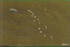 Depicted in
Figure 1 is a macro-seep in the Ballona Channel near Los Angeles, CA which
contains petroleum related gas from a reservoir in the Pico formation at about
2000 feet subsurface. We will discuss the surrounding pattern of micro-seepage
later in this paper, but such a leaking reservoir would no doubt be an
excellent place to monitor the pattern and rate of CO2 seepage
following injection into this subsurface reservoir.
Depicted in
Figure 1 is a macro-seep in the Ballona Channel near Los Angeles, CA which
contains petroleum related gas from a reservoir in the Pico formation at about
2000 feet subsurface. We will discuss the surrounding pattern of micro-seepage
later in this paper, but such a leaking reservoir would no doubt be an
excellent place to monitor the pattern and rate of CO2 seepage
following injection into this subsurface reservoir.
 Before we explore the application
of technology to the carbon sequestration initiative, it is worthwhile to briefly review
the history of the development of seep detection related to petroleum
exploration. The observation of seeps, both macro and micro, is the oldest
method of exploring for oil and gas and several significant historical events
are depicted on Figure 2, including the fact
that the first oil well, the Drake well in Pennsylvania, was drilled on a
macro-seep. Several well known explorationists have observed that a very
significant fraction of the worlds reserves were discovered on the basis of
seep observation, including all of the very large fields discovered as late as
1947 in the middle east (Link, 1952, Hunt, 1983).
Before we explore the application
of technology to the carbon sequestration initiative, it is worthwhile to briefly review
the history of the development of seep detection related to petroleum
exploration. The observation of seeps, both macro and micro, is the oldest
method of exploring for oil and gas and several significant historical events
are depicted on Figure 2, including the fact
that the first oil well, the Drake well in Pennsylvania, was drilled on a
macro-seep. Several well known explorationists have observed that a very
significant fraction of the worlds reserves were discovered on the basis of
seep observation, including all of the very large fields discovered as late as
1947 in the middle east (Link, 1952, Hunt, 1983).
A significant effort was undertaken to characterize petroleum seeps by Gulf Research and Development Company in the 1970’s and 1980’s (Jones, 1976, 1984, Mousseau et al, 1979, Weismann, 1980, Mousseau and Glezen, 1980), (Mousseau, 1981a, 1981b, 1983, Jones and Pirkle, 1981,Jones and Drozd, 1983). Experience derived from that program along with the authors’ subsequent technology forms the basis for this discussion of the application of the petroleum experience to the carbon sequestration program. An important development from the Gulf program was the realization that seeps occur over all petroliferous basins, not only sequestered fluids from the reservoirs, but also fluids that were never sequestered, but migrated vertically from the source rocks at depth. Recently, Larry Cathes at Cornell and Jean Whelan at Woods Hole have suggested that. only 1% of the hydrocarbons generated in source rocks may have been sequestered in commercial fields, with the remaining 99% in some state of vertical migration toward the surface. A News Note by Lisa M. Pinsker published in Geotimes (June, 2003) entitled “Raining Hydrocarbons in the Gulf” provides further details of their recent conclusions regarding seeps.
The observation that the seepage of fluids is pervasive across basins suggests that basins may have pervasive conduits for fluids to migrate to the surface, and that no subsurface structures may be perfect traps. This includes brine filled aquifers in non-commercially petroliferous basins and non petroliferous parts of basins with commercial deposits. Further, the extent of these imperfections will need to be determined and quantified if carbon in the form of carbon dioxide is to confidently be stored subsurface. The lightest of the petroleum fluids, the C1 – C4 hydrocarbons have served as excellent tracers for determining the intersection of vertical conduits of migrating subsurface hydrocarbons and the surface. Since most basins have “source rocks” at depth that have generated such fluids, whether commercial deposits have or have not been discovered, these light gases which are similar in molecular weight and other properties to carbon dioxide, will be the key to identifying conduits of fluid migration above sequestered carbon dioxide.
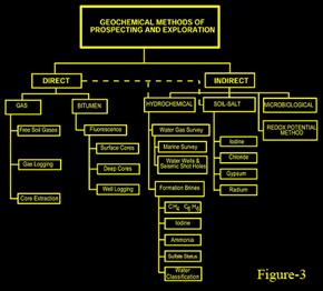 Although many methods have been proposed for mapping petroleum
seeps, as shown in Figure 3, we have determined from our experience that the best and most reliable method is to measure the light C1- C4
hydrocarbons in the free soil gas, with particular emphasis on the ethane through
butanes, since their only source is from thermogenic hydrocarbons at depth.
These light hydrocarbons can be found and collected at measurable
concentrations in the vapor of soil pore spaces at shallow (3 - 6 feet)
depths.
Although many methods have been proposed for mapping petroleum
seeps, as shown in Figure 3, we have determined from our experience that the best and most reliable method is to measure the light C1- C4
hydrocarbons in the free soil gas, with particular emphasis on the ethane through
butanes, since their only source is from thermogenic hydrocarbons at depth.
These light hydrocarbons can be found and collected at measurable
concentrations in the vapor of soil pore spaces at shallow (3 - 6 feet)
depths.
Experience has shown that soil gas extraction can be obtained by pounding a 4 foot hole in the ground, inserting a probe that is connected to a clean evacuated bottle and drawing gas into the bottle under vacuum. The gas can be measured in the field or in a fixed laboratory.
 A typical soil gas probe is, shown in Figure 4, being used
to collect a sample from a depth of
four feet. In such a vapor sample the light, C1
- C4, hydrocarbons concentrations can be measured
down to5 to 10 ppbv. As shown in Figure 4, a soil gas sample is being
collected in a 125 ml glass bottle.
A typical soil gas probe is, shown in Figure 4, being used
to collect a sample from a depth of
four feet. In such a vapor sample the light, C1
- C4, hydrocarbons concentrations can be measured
down to5 to 10 ppbv. As shown in Figure 4, a soil gas sample is being
collected in a 125 ml glass bottle.
The C2 - C4 hydrocarbon gases should always be measured as part of a carbon sequestration seepage program because they provide unique identification of thermogenic-related gases whose source is at reservoir depth or below. Experience has shown that these C2 - C4 gases can serve as natural tracers for the petroleum gases that would migrate from a reservoir used for carbon sequestration. It is important to note here that the presence of carbon dioxide or methane in vadose zone gases does not provide conclusive proof of a vertical migration conduit from depth because these two gases can be produced from the near surface degradation of organic matter. However, significant quantities of the C2 - C4 hydrocarbons are not produced in the near surface soils (except as degradation products in environmental contaminant plumes); thus they can generally be viewed as thermogenic (formed by thermal degradation of organic material at depth) in origin. In addition, the inclusion of C2-C4 gases allows for interpretation of mixed thermogenic, biogenic and sequestered gases, such as methane and CO2, which can have both deep and shallow sources. Measurement ofCO2 and CH4 without normalizing gases, such as C2 - C4 can lead to spurious and un-interpretable results. The presence of correlated (C2 - C4) andCO2 can provide deep source confirmation of the presence of gases of thermogenic and sequestered origin versus gases of biogenic origin.
These conclusions have been confirmed by many major oil company seep detection programs, including very recent research at Shell Global Solutions which has focused on the measurement of ethane in the ambient air as an exclusive indicator for subsurface petroleum deposits (Hirst, et al., 2004). Ethane was selected because it is very light, mobile and is non-biogenic. Shell Global Solutions is currently developing a new airborne ethane gas sensor instrument for exploration. This new instrument can detect 50 parts per trillion in the air. Typical background ambient air ethane concentrations are generally less than 2 ppb, over 40 times greater than the detection limit of this new instrument. This new instrumentation was developed jointly for exploration and medical applications by scientists at the University of Glascow working with and supported by Shell Global Solutions.
Shell’s new ethane instrument could provide a very significant improvement for conducting regional surveys designed to find and detect vertical seepage anomalies over large regional areas before applying soil gas methods. A similar instrument should be possible based on CO2 and could be used to detect anomalous ambient air concentrations of CO2 over carbon sequestration projects areas. However, the soil gas methodology still has many advantages over ambient air measurements, and should always be applied as part of the ground-truth follow-up. Soil gas provides a more precise ground location of any ethane anomalies, and even more importantly, soil gas measurements have the ability to detect other non-biogenic C2 - C4 gases, such as propane and butanes, further confirming the validity and deep-source origins of the ethane measurements. In addition, soil gas data also provides for measurement of any mixed thermo/biogenic gases, such as methane and CO2, which can have both deep thermogenic and shallow biogenic sources.
SOIL GAS ANOMALIES OVER PETROLEUM RESERVOIRS
The Pineview Oil Field Survey
Perhaps the most direct observational evidence with application to the subsurface sequestration of carbon dioxide in petroleum reservoirs is found in examples of soil gas light hydrocarbons, C1 - C4 , over known petroleum reservoirs. While such observations have been made since the earliest days of the petroleum industry as earlier noted, it was during the intense effort at Gulf Research beginning in the 1970’s that correlations between these accumulations and the surface manifestation of migration conduits began to be systematically elucidated.
 An excellent
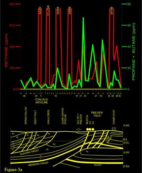
example from our earlier published works is shown in Figure 5a by data from a
soil gas survey conducted in 1976 over the Pineview Oil Field in Wyoming when
the field contained only three producing wells (Jones and Drozd, 1983). This
field produces from the Nugget Formation located 9000 feet below surface. The
data plotted on the profile shown in Figure 5a were collected on 0.25 mile
centers from a depth of 10 feet, and as shown, the soil gas anomaly to
background ratios are very large and unmistakable as anomalies. Methane is
plotted in red and the sum of propane plus butanes are plotted in green. Note
that the methane values, which range upwards to 2000 - 11,000 ppmv (0.2 to
1.1%) have been truncated at 800 ppmv. An idealized cross section of the
geologic structure is shown below the data, with the position of the Pineview
field indicated. It is also significant to note that the green propane plus
butanes profile has it’s largest values between the Elkhorn Thrust on the left
to the Tunp Thrust on the right. This suggests that the oil source lies
within the thrust plate defined by these two faults.
An excellent
example from our earlier published works is shown in Figure 5a by data from a
soil gas survey conducted in 1976 over the Pineview Oil Field in Wyoming when
the field contained only three producing wells (Jones and Drozd, 1983). This
field produces from the Nugget Formation located 9000 feet below surface. The
data plotted on the profile shown in Figure 5a were collected on 0.25 mile
centers from a depth of 10 feet, and as shown, the soil gas anomaly to
background ratios are very large and unmistakable as anomalies. Methane is
plotted in red and the sum of propane plus butanes are plotted in green. Note
that the methane values, which range upwards to 2000 - 11,000 ppmv (0.2 to
1.1%) have been truncated at 800 ppmv. An idealized cross section of the
geologic structure is shown below the data, with the position of the Pineview
field indicated. It is also significant to note that the green propane plus
butanes profile has it’s largest values between the Elkhorn Thrust on the left
to the Tunp Thrust on the right. This suggests that the oil source lies
within the thrust plate defined by these two faults.
This example illustrates the most important conclusion found by GR&DC scientists that the composition of the seeps changes in direct response to the subsurface source, so that seeps characteristic of gas occur over gas fields and seeps characteristic of oil occur over oil fields. This distinction between oil and gas reservoirs can be defined by the ratios of the light C1- C4 gases (Jones and Drozd, 1976, 1983). Details regarding the usefulness of seeps to predict the “oil versus gas” potential have also been discussed Jones and Drozd, 1983 and Jones et al., 2000). This Pineview profile illustrates these compositional changes by the proportion of propane plus butanes relative to methane. To practitioners of petroleum exploration surface geochemistry, this suggests that the potential is greater for liquid hydro carbon production from the Pineview field than in adjacent portions of this survey. To practitioners of carbon sequestration this might suggest that the composition of the fluids migrating vertically from a reservoir is representative of the fluids in the reservoir, and that if compositional fractionation occurs, it is small compared to the overall composition of the fluids.
These compositional differences are further reinforced by the data on the left portion of this soil gas profile (Figure 5a) where the seepage comes from the Coalville Gas Storage reservoir which contains natural gas. Here, the proportion of propane plus butanes to methane is much smaller as would be expected from natural gas as compared to oil. If carbon dioxide were eventually stored in either of these reservoirs, the resulting composition of reservoired hydrocarbons relative to the sequestered carbon dioxide would be unique and would be unmistakable, even when measured in the near surface soil gas.
There is little doubt that the magnitude of the observed seepage in this example is in no small part due to the obvious fault related conduits shown on the geologic cross section, however as we will see later, such large magnitudes are not required to identify migrational conduits. It should be noted that both of these reservoirs are structural in nature and bounded by faults.
Although the Pineview field data plotted on this example was collected from a depth of approximately 10 feet, some shallow soil gas probe samples were also collected as part of our earlier research on soil gas probe methodology. These shallow soil gas samples were collected from only one foot in depth, and although fractionated in composition, they did provide a similar compositional response to the deeper 10 foot deep soil gas data.
 The Pleasant Creek Gas Storage
Field Survey
The Pleasant Creek Gas Storage
Field Survey
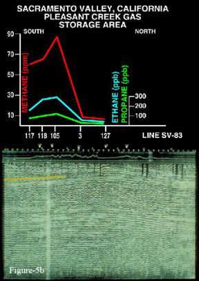
Shown on Figure 5b is a line of soil gas data, again from a depth of 10 feet at 0.25 mile spacing, over the Pleasant Creek Gas storage field in California. This gas storage reservoir is a shallow stratigraphic trap, truncated at the top of the Cretaceous section at a depth of 760 m (2,500 ft) (Hunter, 1955). The reservoir was filled to capacity with a pressure of 10,343 kPa (1,500 psi) when the soil gas data was collected and analyzed. Because this area naturally contained only dry gas, the filling of an abandoned gas sand with pipeline natural gas cannot be expected to change appreciably the composition of surface soil gases. However, the injected storage gas would maintain the subsurface pressure and keep the vertical migration avenues charged. Although no fault-related migrational conduits are obvious, there are still some unmistakable soil gas anomalies which reflect the composition of the natural gas stored in this reservoir. The compositional repeatability of soil-gas surveys conducted over this Pleasant Creek Gas Storage Field is demonstrated by the following data.
|
Date |
C1/∑Cn |
C1/C2 |
(C3/C1) x 1,000 |
|||||
|
|
|
|
|
|||||
|
May 1975 |
90 |
20 |
19 |
|||||
|
July 1975 |
89 |
18 |
24 |
|||||
|
July 1976 |
89 |
16 |
20 |
|||||
|
|
|
|
|
|||||
 The Hartzog Draw Oil Field
Survey
The Hartzog Draw Oil Field
Survey
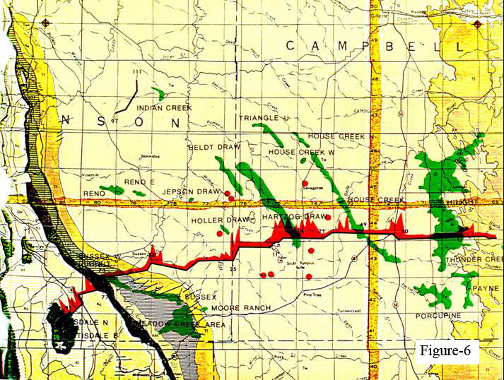
An example from the Powder River Basin in Wyoming that was collected in 1976 is shown in Figure 6. This example serves to illustrate that a single line of soil gas data across several producing trends was able to identify several of the producing reservoirs. The objective of this survey was to evaluate a prospect within an area of unknown potential near Pumpkin Buttes, Wyoming where no fields had been discovered at the time of the survey. Clearly there are magnitude anomalies coincident with what is now the Hartzog Draw field, which produces from a barrier island “Shannon” sandbar located at a depth of 9000 feet below the surface. This field, discovered after the soil gas survey was completed, is the second largest field in the Powder River Basin. This discovery was predicted by the geochemical survey, and the field was confirmed approximately one year after the soil gas survey was completed.
 The Marquez Field Survey
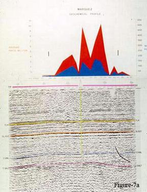
Shown on Figure 7a is the Marquez field in Limestone Co. Texas which was discovered by a soil gas survey conducted in 1979. This anomaly lies directly over the Marquez field which produces from the Cotton Valley formation at a depth of 12,000 feet.
The Weyland Oil Field Survey
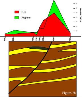
Shown on Figure 7b is data from a soil gas survey conducted over the Weyland Oil Field in Cass County Texas. Notice that the soil gas anomaly is deflected somewhat by the bounding growth fault so that it is not observed directly over the reservoir. Also significant is the fact that the oil reservoired in the Weyland field is of high sulfur content and H2S was found in soil gas in the surface samples. This is a significant example in that H2S is much more reactive, sorptive and soluble than typical soil gas C1-C4 hydrocarbons, yet H2S can survive the migration path from reservoir to the surface. This example provides little doubt that carbon dioxide will also survive similar migrational paths.
 In the examples cited to this
point, soil gas magnitudes were significantly above the background levels
measured in the areas being surveyed. Such large signal to background ratios
are not required if the monitored species is carefully chosen. Recall that we
have discussed that methane can have two sources, one thermogenic and related
to depth and one biogenic and related to near surface processes. We have
suggested that in some cases the most prudent course is to place more confidence
in the C2-C4 hydrocarbons, at least for initial data
interpretation. When considering the natural abundance of these hydrocarbons,
it is useful to point out that both in the reservoir, and in their associated
surface seepages, C2 > C3 > C4. . In the
near-surface where the concentrations of these hydrocarbons are very low the
heavier components, such as butanes, and even propane may fall below the
analytical detection limits. In such cases, one may have to rely on the
largest component (ethane) as the main indicator. The following example, shown
in Figure 8 has used the latter approach of monitoring only C2.
In the examples cited to this
point, soil gas magnitudes were significantly above the background levels
measured in the areas being surveyed. Such large signal to background ratios
are not required if the monitored species is carefully chosen. Recall that we
have discussed that methane can have two sources, one thermogenic and related
to depth and one biogenic and related to near surface processes. We have
suggested that in some cases the most prudent course is to place more confidence
in the C2-C4 hydrocarbons, at least for initial data
interpretation. When considering the natural abundance of these hydrocarbons,
it is useful to point out that both in the reservoir, and in their associated
surface seepages, C2 > C3 > C4. . In the
near-surface where the concentrations of these hydrocarbons are very low the
heavier components, such as butanes, and even propane may fall below the
analytical detection limits. In such cases, one may have to rely on the
largest component (ethane) as the main indicator. The following example, shown
in Figure 8 has used the latter approach of monitoring only C2.
 The Kansas – Colorado
State Line Complex Survey
The Kansas – Colorado
State Line Complex Survey
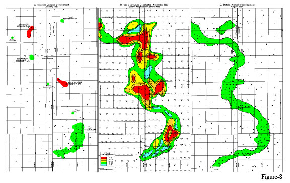
A reconnaissance soil gas survey was conducted on the Kansas-Colorado border in November 1987 over an area of 150 square miles as shown in the center section of Figure 8. Plotted are soil gas ethane magnitudes which were found in the range of 10 – 30 ppbv. The Stateline Complex is on the northeast flank of the northeast plunging Las Animas Arch, which separates the Denver Basin to the northwest from the Hugoton Embayment to the southeast. Production is from stratigraphic traps at depths ranging from 5000 to 5500 feet in the Lower Pennsylvanian Johannes and Stockholm members of the Morrow Formation. In 1979, TXO drilled the discovery well for the SW Stockholm Field (and the Stateline Trend) at the location shown on left portion of Figure 8. At this time, there were only four fields in the immediate area. There were two one-well abandoned Mississippian oil Fields (Funk and Encampment Fields) and two Morrow gas fields (Arapahoe and W Stockholm Fields). These four fields were discovered as a result of various exploration plays on low-relief structures.
By the end of 1986, the SW Stockholm Field had been developed to the extent shown on the left portion of Figure 8. The field contained 53 wells and extended for four miles. During 1987 there were three significant developments in the area: (1) TXO completed a one-half mile field-extension in March with the Wallace # 1-R; (2) in April 1987, Medallion drilled a Morrow oil new field discovery with the Arapahoe # 27-1 eight miles to the north of SW Stockholm Field; (3) in July 1987, Mull Drilling established a Morrow oil new field discovery with the Stateline Ranch # 1 well four miles north of SW Stockholm Field. These three wells, along with the wells of SW Stockholm Field had, in general terms, defined a Morrow sand oil fairway for a distance of 10 miles in a north-south direction (see left portion of Figure 8). Based on these discoveries, a decision was made to conduct a reconnaissance surface soil gas survey in the area. Subsequent exploration and development drilling has delineated a complex of nine Morrow Sand fields over 25 miles long (see right portion of Figure 8) consisting of over 270 wells which have a cumulative production of over 12 MMBO. It can be clearly seen that as early as 1987, the soil gas survey had accurately defined the general areal extent of the productive Morrow incised valley as would be confirmed by development drilling three years later in 1990 (see right portion of Figure 8). A detailed discussion of this example is available. (Dickinson et al., 1994, Jones and LeBlanc, 2004, LeBlanc and Jones 2004a and 2004b).
These are just a few of the examples that are available for demonstrating the use and value of soil gas surveys for finding natural micro- and macro-seepage conduits associated with petroleum reservoirs. As these examples show, migrational conduits need not generate large near surface anomalies in order to be detectable, and even more important, they demonstrate one of the most important conclusions concerning surface prospecting methods, which is that there is no relationship between the magnitudes of seeps and the volume of fluid contained in the associated subsurface reservoir. In the case of carbon dioxide, which for carbon sequestration evaluation will have both a biogenic source in the near surface and a potential source at depth, evaluation of migrational conduits will be significantly aided by detailed background surveys prior to injection.
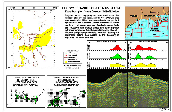
Mapping of seepage is not limited to “onshore” reservoirs, but can be implemented in offshore basins as well, as shown on Figure 9.
 The Joliett Field Drop Core
Survey
The Joliett Field Drop Core
Survey
In this example drop core samples were collected in 1983 over the area where the Joliett field was later discovered in the Green Canyon area of the Gulf of Mexico. Gas containing 100% hydrocarbons and pockets of free oil were found in near surface core samples. This example further reinforces the fact that the magnitude of seepage is not related to the volume of reservoired fluid, but rather to fluid pressure drive and permeability along the migration path. Fluids here were found in near surface cores, however anomalous concentrations of gas are regularly found in the water column above many offshore petroleum reservoirs.
 The Gulf Marine Geochemical
“Sniffer” Detector
The Gulf Marine Geochemical
“Sniffer” Detector
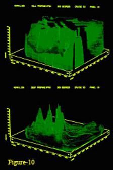
GR&DC scientists designed, built, and operated several marine seep detectors, sometimes called “sniffers”, which were employed aboard various research vessels, such as the R/V HOLLIS HEDBERG, along with its predecessor, the R/V GULFREX (Mousseau and Williams, 1979, Mousseau and Glezen, 1980), (Mousseau, 1981a, 1981b, 1983). These ships conducted extensive and detailed surveying over continental shelves worldwide and particularly the Gulf of Mexico (Mousseau et al, 1979). The R/V HOLLIS HEDBERG system employed three separate water inlets which continually supplied sample streams from the near surface, from intermediate depths to 450 feet and from a depth of 565 ft. while the ship was underway at normal seismic survey speeds. Each sample stream was analyzed for seven (7) hydrocarbon gases once every three minutes with a sensitivity which depends upon the hydrocarbon, but for example, is about 50 picoliters of propane at STP per liter of seawater. The purpose for using three inlets was to differentiate between surface contamination and seepage. As shown in Figure 10, which is a 3-D perspective plot of propane from the hull and deep inlets, surface contamination can be a major interference to shallow sampling, but is not a factor in identifying seeps using the deep inlet.
Hedberg Rules! - Gulf Science & Technology Company - (Gulf Oilmanac 6-80, pp. 2-4) - http://eti-geochemistry.com/oilmanac680/index.html
 Marine Anomalies and
Brightspots
Marine Anomalies and
Brightspots
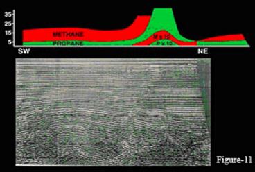
The most typical form in which the "sniffer" data was deployed when used in conjunction with seismic as an exploration tool is illustrated in Figure 11 (Mousseau and Williams, 1979, Weismann, 1980). Geochemical data from a deep tow inlet in profile form is shown superimposed to scale on a seismic record. Such records were produced at sea by Gulf to aid the explorationist in making real time evaluations of hydrocarbon potential of structurally significant areas. The anomaly represented in Figure 11 is considered a "localized" anomaly because of the relatively short duration of the hydrocarbon signal and the magnitude of the hydrocarbon concentrations relative to regional background. Several "bright spots" may be seen on the seismic section at depth as well as shallow gas-charged sands presumably sourced by migration along the observed fault plane.
 The High Island
Surveys
The High Island
Surveys
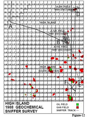
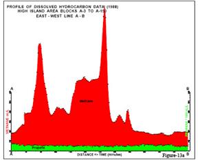
In another example, a marine hydrocarbon seep detection survey was completed over High Island Blocks 152A and 198A and surrounding areas in April, 1988, as shown in the site location track map on Figure 12 (Jones et al., 1988, Jones et al., 2000). This study, consisting of 239 miles of sniffer data, was conducted aboard the RV/GYRE by Texas A&M University, in conjunction with Exploration Technologies, Inc., using the marine hydrocarbon analytical system originally designed by Gulf as earlier described. Light hydrocarbon data were collected continuously along seismic lines of interest from a water sampling system towed about 30 feet above the bottom of the sea floor. A total of 52 miles of gridded data (259 analyses) were completed over the Block 152 study area and a total of 31 miles of gridded data (129 analyses) were completed over the Block 198 study area at 3 minute intervals giving an approximate sample spacing of about 1500 feet. Three regional profiles are included as Figure 13a, 13b, and 13c to show the magnitude variations along the survey lines.
 Survey tracks,
as shown on Figure 12, include a 54 mile long regional north-south line which
extends from Block 198 down to Block 321 in the High Island South extension. This
regional line plotted on Figure 13b, provides both a calibration data set over
the known gas fields and a background data set which extends between the two
gridded blocks. As shown by Figure 13b, background values are observed in
Blocks 237, 224, and 223 where methane drops down to about 100 nl/l, ethane is
below 0.70 nl/l, and propane is below 0.50 nl/l. These thresholds are typical
of Gulf of Mexico backgrounds from previous study data (Mousseau and Williams
1979).
Survey tracks,
as shown on Figure 12, include a 54 mile long regional north-south line which
extends from Block 198 down to Block 321 in the High Island South extension. This
regional line plotted on Figure 13b, provides both a calibration data set over
the known gas fields and a background data set which extends between the two
gridded blocks. As shown by Figure 13b, background values are observed in
Blocks 237, 224, and 223 where methane drops down to about 100 nl/l, ethane is
below 0.70 nl/l, and propane is below 0.50 nl/l. These thresholds are typical
of Gulf of Mexico backgrounds from previous study data (Mousseau and Williams
1979).
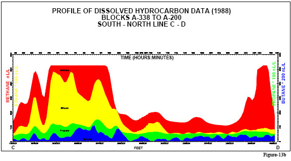 The largest magnitude anomalies
observed on this entire survey, are also noted on this regional line (Figure
13b), where it crosses the center of Block 268 and traverses the major trend of
the known gas producing fields. Within this producing trend, methane goes over
500 nl/l, ethane ranges from 1-2 nl/l up to 5 nl/l, and propane rises from 0.50
to 1 nl/l. In addition, as shown on Figure 13c, iso and normal butane reached a
combined total of about 1 nl/l in anomalies associated with these known gas
fields.
The largest magnitude anomalies
observed on this entire survey, are also noted on this regional line (Figure
13b), where it crosses the center of Block 268 and traverses the major trend of
the known gas producing fields. Within this producing trend, methane goes over
500 nl/l, ethane ranges from 1-2 nl/l up to 5 nl/l, and propane rises from 0.50
to 1 nl/l. In addition, as shown on Figure 13c, iso and normal butane reached a
combined total of about 1 nl/l in anomalies associated with these known gas
fields.
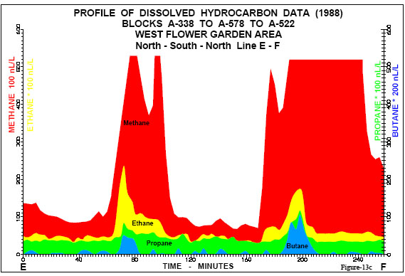
The presence of butanes in the sniffer data clearly separates the southerly gas producing trend from that data gathered to the north of Block 252. Both the grids over Blocks 152 and 198 and the profile data north of Block 252 as shown by Figure 13a, exhibit a clear lack of propane and butane anomalies. The presence of mainly methane in the northern areas suggests that these anomalies are derived from biogenic gas sources.
Marine compositional crossplots from the anomalies observed in Block 152 and 198, and from the regional profile fall exactly as expected, based on the known oil and gas producing reservoirs within this survey area. Both Blocks 198 and 152 are similar to the fairly dry gas type Pleistocene reservoirs found in West Cameron in the Louisiana offshore and are indicative of only gas potential. Block 198 sniffer anomalies appear to contain even drier (greater proportion of methane relative to (C2-C4)) gas data than Block 152. In contrast, compositions measured in both of these blocks are slightly oilier increased proportion of (C2-C4) relative to methane) than the major Pliocene gas producing trend which lies to the south of Blocks 152 and 198. The increase in ethane, propane, and butanes in this southern gas producing area suggest that these gas fields in the southern part of the area surveyed contain Pliocene gas from a more petrogenic source, whereas the areas to the north appear to be dominated by biogenic gas sources which don't contain C2 plus components. It should be noted that the new field discoveries (A-129, A-154 and A-200) highlighted on Figure 12 were made after the sniffer survey was completed. Additional details regarding the composition correlations are contained in Appendix A.
It is probable that were carbon dioxide sequestered in offshore petroleum reservoirs, anomalous concentrations would be detectable in the overlying water column if significant reservoir leakage occurred.
While carbon sequestration targets will always be discrete, well defined reservoirs at depth, the results of basin wide surveys for petroleum related C1 - C4 hydrocarbons provide a very important perspective with regard to the pervasiveness and repeatability of natural hydrocarbon seepage. As noted and discussed earlier, natural micro- and macro- seeps originate from both the reservoirs and the source rocks that generated the reservoired petroleum. This relationship with the source rocks provides coherent compositional signatures that are basin wide, rather than just reservoir focused, as will be the case with sequestered CO2. This basin-wide characteristic of natural hydrocarbon seepage provides both stability and compositional coherence that not only allows prediction of “oil versus gas” sources, but also allows recognition of biogenic methane and CO2 soil gases related to vadose zone contamination sources. Biogenic methane and CO2 gases derived from such shallow sources not only have very large C1/C2 ratios (> 1000), but they also are very small in areal extent when compared to natural seepage. The average contamination plume from a gasoline station is only 250 feet in extent, and only very rarely do such contaminant plumes extend 3000 to 5000 feet. Natural seeps, on the other hand extend over several miles (over entire basins) with no significant changes in composition. By conducting both regional and detailed surveys, this “source rock” information can be used to properly catalog and classify specific seeps that might be related to a particularreservoir that has been selected for CO2 sequestration. This is a very important consideration because CO2 sequestration will be carried out within old fields, where old spills and casing and pipeline leakages will have occurred. In most cases the fields selected for sequestration of CO2 will have contamination that must be characterized when measuring and interpreting their vadose zone gases.
 Many examples
demonstrating the repeatability of both the composition and magnitudes of
natural seeps are available in Appendix A (Jones and Drozd, 1983, Jones and
Burtell, 1996, Jones et.al. 2000), however some of the best examples ever
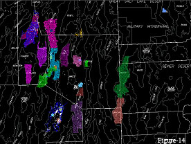
gathered are shown by surveys conducted within the Great Basin in Nevada. Over
the last 30 years ETI has collected over 12,212 soil gas samples (see Figure
14) on regional one mile spaced grids (on section corners and centers) over
many of the individual basins in Nevada. The data come from thirteen Great
Basin valleys, including Pine and Railroad valley’s where commercial
accumulations have been discovered. This Nevada soil gas data exhibits both
spatial and compositional clustering with anomalies highlighting all of the known
fields and clearly demonstrates the stability and repeatability of the data.
Such regional surveys provide a very good measure of both compositional
stability and anomaly location because the data covers the entire basin,
including productive trends and background areas displaced from productive
trends. Published Railroad Valley case studies conducted in 1984 – 85 are
available (Jones et al.1985, 1986,2000)
in Appendix A.
Many examples
demonstrating the repeatability of both the composition and magnitudes of
natural seeps are available in Appendix A (Jones and Drozd, 1983, Jones and
Burtell, 1996, Jones et.al. 2000), however some of the best examples ever
gathered are shown by surveys conducted within the Great Basin in Nevada. Over
the last 30 years ETI has collected over 12,212 soil gas samples (see Figure
14) on regional one mile spaced grids (on section corners and centers) over
many of the individual basins in Nevada. The data come from thirteen Great
Basin valleys, including Pine and Railroad valley’s where commercial
accumulations have been discovered. This Nevada soil gas data exhibits both
spatial and compositional clustering with anomalies highlighting all of the known
fields and clearly demonstrates the stability and repeatability of the data.
Such regional surveys provide a very good measure of both compositional
stability and anomaly location because the data covers the entire basin,
including productive trends and background areas displaced from productive
trends. Published Railroad Valley case studies conducted in 1984 – 85 are
available (Jones et al.1985, 1986,2000)
in Appendix A.
Pine Valley Surveys
These surveys were conducted as exploration products for many of the major oil companies in the US. Repeating a survey essentially doubles the cost, and is, therefore rarely done. On one occasion, however, the natural competitive environment generated by free enterprise exploration between these major oil companies presented an opportunity to collect two very large regional exploration data sets of approximately 1000 samples each in Pine Valley, Nevada. The Pine Valley data were collected as two independent data sets from a depth of 4 feet. The first data set was collected in 1986 and contains 1007 soil gas sites and the second was collected in 1988 and contains 985 soil gas sites. Both surveys were collected before GPS was available, so all locations were determined by map and compass by the same geologist. Thus, these surveys provide two independent and unbiased data sets that attempt to measure the same regional seepage patterns. A statistical comparison between these two sets of data is shown below.
|
Project |
|
Survey A |
Survey B |
|
Year |
|
1986 |
1988 |
|
(Total Samples) |
|
(1007 sites) |
(985 sites) |
|
|
|
|
|
|
Methane (ppmv) |
|
0.925 |
1.320 |
|
Ethane (ppmv) |
|
0.020 |
0.027 |
|
Propane (ppmv) |
|
0.015 |
0.016 |
|
|
|
|
|
|
C1/C2 Ratio |
1st quartile |
103.0 |
112.0 |
|
|
2nd quartile |
46.8 |
46.8 |
|
|
3rd quartile |
21.6 |
20.6 |
The very low median concentrations of 20 ppbv versus 27 ppbv for ethane and 15 ppbv versus 16 ppbv for propane in Surveys A and B respectively, indicate that 50 % of the samples (approximately 500 samples out of each data set) have concentrations, near background, yet the anomalies are the same on both surveys. Let us look further at the compositional signatures expressed by this data. Note the repeatability of the methane/ethane quartiles. The median C1/C2 ratio is 46.8 on both surveys, which were conducted two years apart. The upper and lower quartiles are also very similar. As noted earlier, soil gas data can predict the oil versus gas potential of an unknown basin through the compositions of the light gases (Jones and Drozd, 1983). This compositional relationship of soil gas to the gases generated within the basins surveyed is its most valuable asset. This allows recognition of valid migrated gas seeps and provides a framework for defining seep locations for future monitoring of reservoir gases.
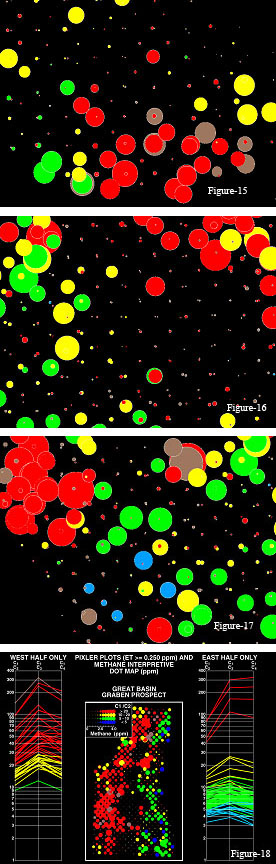 This Pine Valley
data set provides a unique opportunity to demonstrate the reproducibility of
both magnitude anomalies and regional composition as measured by vertically
migrating hydrocarbons at the surface. Shown on Figures 15, 16 and 17 are
pairs of soil gas samples within small areas of the Pine Valley dataset. At
each location there are two samples. Within the background or low magnitude
areas there is very little variation and magnitudes repeat fairly well. The
magnitude anomalies exhibit considerably more variation. The higher magnitude
anomalies cluster in the same areas relative to background in both the 1986 and
1988 data sets. The repeatability and clustering of sample composition is also
well demonstrated on this scale.
This Pine Valley
data set provides a unique opportunity to demonstrate the reproducibility of
both magnitude anomalies and regional composition as measured by vertically
migrating hydrocarbons at the surface. Shown on Figures 15, 16 and 17 are
pairs of soil gas samples within small areas of the Pine Valley dataset. At
each location there are two samples. Within the background or low magnitude
areas there is very little variation and magnitudes repeat fairly well. The
magnitude anomalies exhibit considerably more variation. The higher magnitude
anomalies cluster in the same areas relative to background in both the 1986 and
1988 data sets. The repeatability and clustering of sample composition is also
well demonstrated on this scale.
Snake Valley Surveys
Shown on Figure 18 is a petroleum related soil gas data set, collected at a depth of 4 feet, over the entire basin in Snake Valley, Nevada where no commercial wells have yet been drilled. Samples were again collected on section corners and in the middle of each section. Note that there are measurable concentrations of C1-C4 hydrocarbons in every sample, in spite of the fact that there are no commercial fields discovered to date. As noted above, the average contaminant plume of a gas station site in the US is only 250 feet and man made plumes longer than one mile are rare. Only a source rock at depth could be responsible for the presence of these measured hydrocarbons, which clearly exhibit stable, but regionally controlled compositions. Our worldwide soil gas data has demonstrated that the regional differences in composition are related to source rock thermal history or maturity, and not to compositional fractionation during vertical migration. This suggests with regard to carbon sequestration that seeping carbon dioxide, when detected, can be normalized by the regional hydrocarbon compositions, even within a basin like Snake Valley where commercial production has not yet been discovered. These examples demonstrate that in all basins, the migrational conduits can be characterized a-priori by the presence of C1 - C4 hydrocarbons. At the same time that these hydrocarbon seeps are being measured, the background carbon dioxide in the area around the target reservoir can also be established. Both are essential for recognition of carbon sequestration related seepage.
The example shown in Figure 18 is not an isolated case. During early development of these concepts at Gulf Research, a 600 site survey conducted in the Permian Basin in 1976 confirmed this compositional stability. This survey area was actually sampled twice with the second set of samples located halfway between the first set of samples. Such results served to demonstrate the widespread seepage, and in particular, the compositional stability of the regional hydrocarbon seepage patterns. These early observations were established in both California and West Texas surveys were presented at the 1976 AAPG meeting and were published (Jones and Drozd 1983).
These results demonstrate that seeps are not only related to reservoirs, but occur basin wide, because of their relationship to the source rocks at depth. As previously noted, the vertical migrational conduits are controlled by basin dynamics. While these widely spaced surveys illustrate the pervasiveness of the conduits, within the area of a target reservoir, much more closely spaced samples will greatly enhance their definition. It also suggests that essentially no reservoirs are perfect traps, and there generally are seeps connected to the surface by vertical migrational conduits which can be defined by soil gas surveys. The most important gases to measure are the C1 - C4 hydrocarbons and the natural levels of carbon dioxide. Proper baseline surveys will significantly enhance the ability to determine leakage of carbon dioxide following sequestration.
Several of our experiences enable us to discuss more definitively the subjects of migrational conduits and the flux of fluids within these conduits.
 Wyoming Underground
Coal Gasification Reactor Monitoring
Wyoming Underground
Coal Gasification Reactor Monitoring
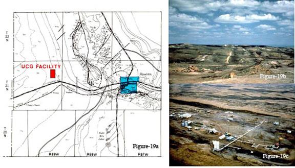
An excellent example was provided in 1981 when Gulf entered into a joint agreement with the Department of Energy to gasify coal in steeply dipping beds in an area near Rawlings, Wyoming (Jones and Thune, 1982, Jones, 1983). The North Knobs UCG facility is located approximately eight miles west of Rawlins in south-central Wyoming (Figure 19a).
 It is situated
on the southwest flank of the asymmetrical Rawlins uplift adjacent to the Washakie
Basin. On Figure 19b are shown (looking north) the steeply dipping (70
degrees) coal and sandstone beds, however only the sandstones outcrop due to
weathering. The well exposed resistant sandstones all exhibit a remarkably
consistent and well developed near-rectilinear joint pattern. The dominant
(systematic) joint set strikes about 6º (N14ºW) from the strike of the beds
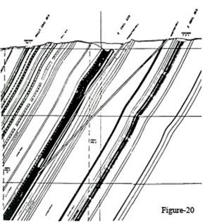
(N20ºW). The picture in Figure 19c is looking to the west. A cross section of
the steeply dipping coal and sandstone beds is shown on Figure 20. To gasify
the coal, a retort was constructed through two near vertical wells and a fire
was started in the subsurface retort cavity to produce combustible gases. It
is perhaps significant to note that the specific composition of the combustion
gases, which include methane, hydrogen carbon dioxide and carbon monoxide, are
perhaps grossly similar to gases which will be produced in the new IGCC power
plants. Gulf Research had completed a previous burn (Burn I) at this site two
years earlier in a retort which was located at a depth of 600 feet subsurface.
This previous burn resulted in extensive gas leakage to the surface, and both
the DOE and Gulf engineers were interested in determining the sources of the
leaks and in making more accurate flux measurements of the resulting seepage.
The second retort was located along strike and about 400 feet deeper than Burn
I in an attempt to reduce the near-surface leakage. Burn I was located nearly
directly below wells Iw-1/Iw-2 and the second burn (Burn II) was located nearly
directly below wells IW-2-2/Iw-2-3.
It is situated
on the southwest flank of the asymmetrical Rawlins uplift adjacent to the Washakie
Basin. On Figure 19b are shown (looking north) the steeply dipping (70
degrees) coal and sandstone beds, however only the sandstones outcrop due to
weathering. The well exposed resistant sandstones all exhibit a remarkably
consistent and well developed near-rectilinear joint pattern. The dominant
(systematic) joint set strikes about 6º (N14ºW) from the strike of the beds
(N20ºW). The picture in Figure 19c is looking to the west. A cross section of
the steeply dipping coal and sandstone beds is shown on Figure 20. To gasify
the coal, a retort was constructed through two near vertical wells and a fire
was started in the subsurface retort cavity to produce combustible gases. It
is perhaps significant to note that the specific composition of the combustion
gases, which include methane, hydrogen carbon dioxide and carbon monoxide, are
perhaps grossly similar to gases which will be produced in the new IGCC power
plants. Gulf Research had completed a previous burn (Burn I) at this site two
years earlier in a retort which was located at a depth of 600 feet subsurface.
This previous burn resulted in extensive gas leakage to the surface, and both
the DOE and Gulf engineers were interested in determining the sources of the
leaks and in making more accurate flux measurements of the resulting seepage.
The second retort was located along strike and about 400 feet deeper than Burn
I in an attempt to reduce the near-surface leakage. Burn I was located nearly
directly below wells Iw-1/Iw-2 and the second burn (Burn II) was located nearly
directly below wells IW-2-2/Iw-2-3.
In order to properly monitor the leakage patterns and the flux, the geochemistry group scientists at Gulf Research installed 122 permanent monitoring wells to a depth of 18 feet subsurface. These stations were placed over, updip and downdip from the subsurface retort. All geochemical monitoring points were created with a 3 inch auger to a nominal depth of 18 feet. Groundwater was not encountered in any of the monitoring points. Each monitoring point was established as a "permanent" observation point by installing a 20 foot length of 1 inch ID PVC pipe which was perforated with about 30 one-quarter inch diameter holes in the lower 1-1 1/2 feet of the pipe. During installation, sufficient pea gravel was poured into the annulus to fill the lower 2 feet. This pea gravel provides a permeable zone for collection of soil gases leaking from the adjacent formations. The remainder of the open hole was backfilled with soil and tamped. Metal tags with the point number were then attached and a removable cap placed on the top of the PVC pipe.
After installation, each monitoring point was allowed to stand for a minimum of 48 hours before sampling, thus permitting the indigenous gases remaining in the hole after drilling to come to equilibrium. All points were then sampled at least twice before any test pressuring or other work on the facility took place. Thus the composition and magnitudes obtained from these samples provide a set of "baseline" data, giving values at each monitoring point prior to any Burn II retort activity. A second full suite of samples (generally more than one from each site) was also taken during the pre-burn air-pressuring of the Burn II production facilities. During this period air pressures reaching 700-800 pounds per square inch were applied to the system, including the focal point in the coal seam. Geochemical near-surface soil-gas sampling during this test period permitted a preview, under maximum operating conditions, of the effective transmissibility of the residual gases through the rocks surrounding the retort of Burn II. This included an opportunity to look for, prior to the ignition of Burn II, any possible preferred migration paths through which product gases might later travel and escape to the surface. After ignition of Burn II, a third sequence of sampling was initiated. This sampling period extended throughout the full interval of the production burn and continued during the shutdown and post-burn period.
Sampling during the burn and post-burn phase of Burn II included periodic resampling of all geochemical sites, with more frequent resampling of those sites that showed changes in composition and/or concentration. The post-burn sampling was carried out in order to see how long the effects of the burn could be detected in the near surface and/or to evaluate the rate of decline of values resulting from the burn.
The analytical measurements were made with three Gulf Research mobile field trucks, in which were gas chromatographs equipped with a flame ionization detector (FID) specially constructed by Gulf Research for light hydrocarbon measurements and an infrared CO2 detector. One of the trucks contained a gas chromatograph equipped with dual FID and TC (thermal conductivity) detectors. The TC detector can measure helium and hydrogen while the FID is used to detect light hydrocarbons. This truck was also equipped with an infrared CO detector and a gas chromatograph with a flame photometric detector (FPD) for measurement of the sulphur gases COS, H2S, CS2 and SO2. During the course of this experiment it was established that the hydrocarbons were completely adequate to define all leakage avenues.
 Because of the
time required to make each set of measurements and the need to periodically
sample 122 individual stations, it was not possible to continuously make
measurements from each monitoring station. In making an analysis of all of the
near- surface hydrocarbon data, it was thought best to prepare a series of maps
based upon the "arrival" times in the near surface which occurred
after each change in the burn system. A statistical analysis was made to
determine the time when the effects of these changes were best recognized.
Comparison of these times with the times when each activity began, with the
exception of the post-burn interval, indicates a realistic figure of
approximately 3 - 5 days for the response to be observed. An examination of
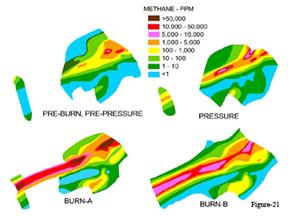
the change in methane flux from various sites suggested that the data could be
divided into at least four discrete periods for mapping and discussion
purposes: (1) Pre-pressure -- July 22, 1981, through August, 16, 1981; (2)
pressure -- August 17, 1981, through August 23, 1981; (3) burn -- August 24,
1981, through November 10, 1981; (4) post-burn -- November 11, 1981, through
December 12, 1981 (end of field survey). On Figure 21, the main changes in
methane concentrations for these four periods are shown.
Because of the
time required to make each set of measurements and the need to periodically
sample 122 individual stations, it was not possible to continuously make
measurements from each monitoring station. In making an analysis of all of the
near- surface hydrocarbon data, it was thought best to prepare a series of maps
based upon the "arrival" times in the near surface which occurred
after each change in the burn system. A statistical analysis was made to
determine the time when the effects of these changes were best recognized.
Comparison of these times with the times when each activity began, with the
exception of the post-burn interval, indicates a realistic figure of
approximately 3 - 5 days for the response to be observed. An examination of
the change in methane flux from various sites suggested that the data could be
divided into at least four discrete periods for mapping and discussion
purposes: (1) Pre-pressure -- July 22, 1981, through August, 16, 1981; (2)
pressure -- August 17, 1981, through August 23, 1981; (3) burn -- August 24,
1981, through November 10, 1981; (4) post-burn -- November 11, 1981, through
December 12, 1981 (end of field survey). On Figure 21, the main changes in
methane concentrations for these four periods are shown.
As noted above, during field operations it was observed that it took approximately 3 to 5 days after the beginning of the system air-pressure test, or ignition of the coal, before any significant increases in the magnitude of the hydrocarbon gases were recognized in the near surface. In the case of the beginning of the post-burn period no precisely observable cutoff date could be defined. From the data it was noticed that on, or about, September 26 most sample sites showed somewhat decreasing soil-gas values. This date is well in advance of burn shutdown, but because there was no large decrease in values after shutdown was initiated, it was thought best to include a map showing the more or less gradual decrease in soil-gas values observed over the period of September 30 through December 12. It is believed that the gradual decrease observed is due to a general lessening of air pressure on the retort after the burn was fully established. As an explanation for the lack of a recognizable decrease shortly after shutdown was accomplished, it is believed that sufficient gases were still in the retort area and the migration paths so completely saturated that "bleeding" of the product gases would continue for an extended period at the relatively low final retort pressure (~ 30 psi).
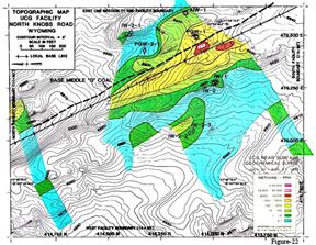 Shown in Figure
22 is the first composite set of data collected from the monitoring network
approximately 2 years after Burn I. These data are pre-burn and
pre-pressurization for the deeper Burn II. The anomalies to the top right are
residual gases remaining from Burn I. As much as 1000 ppm of carbon monoxide
persisted in these strata for 2 years after the end of Burn I.
Shown in Figure
22 is the first composite set of data collected from the monitoring network
approximately 2 years after Burn I. These data are pre-burn and
pre-pressurization for the deeper Burn II. The anomalies to the top right are
residual gases remaining from Burn I. As much as 1000 ppm of carbon monoxide
persisted in these strata for 2 years after the end of Burn I.
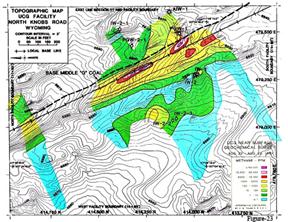 Shown on Figure
23 is data taken after a pressure of 700 psi was applied to the Burn II retort,
but before the burn was initiated. The seep at the coal seam updip of the
Burn II retort is very large and there is also a small increase in seepage at
the far western edge of the coal outcrop. This laterally displaced seep
occurred in time only a few hours after the direct updip seep at the outcrop,
even though the subsurface migration pathway is longer by perhaps 1500 feet.
The surface expression of the seepage occurs within a sandstone bed that
directly overlies the coal bed rather than at the coal outcrop. There is also
a vertical seepage directly above the Burn II retort which is located 1000 feet
below the surface, even though the inclined bedding planes would be expected to
deflect most of the seepage along the bedding planes. Designation of Burn A
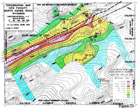
(figure 24) and Burn B (Figure 25) were chosen to distinguish two sequential
time periods during Burn II. Burn A concentration maps show the leakage in the
monitoring stations early during Burn II. Burn B concentration maps show the
leakage in the monitoring stations in later stages of Burn II. The Burn A map
shows composite data collected between Aug. 30 – Sept. 25, 1981 and the Burn B map shows data composited between Sept 26 – Dec 12, 1981.
Shown on Figure
23 is data taken after a pressure of 700 psi was applied to the Burn II retort,
but before the burn was initiated. The seep at the coal seam updip of the
Burn II retort is very large and there is also a small increase in seepage at
the far western edge of the coal outcrop. This laterally displaced seep
occurred in time only a few hours after the direct updip seep at the outcrop,
even though the subsurface migration pathway is longer by perhaps 1500 feet.
The surface expression of the seepage occurs within a sandstone bed that
directly overlies the coal bed rather than at the coal outcrop. There is also
a vertical seepage directly above the Burn II retort which is located 1000 feet
below the surface, even though the inclined bedding planes would be expected to
deflect most of the seepage along the bedding planes. Designation of Burn A
(figure 24) and Burn B (Figure 25) were chosen to distinguish two sequential
time periods during Burn II. Burn A concentration maps show the leakage in the
monitoring stations early during Burn II. Burn B concentration maps show the
leakage in the monitoring stations in later stages of Burn II. The Burn A map
shows composite data collected between Aug. 30 – Sept. 25, 1981 and the Burn B map shows data composited between Sept 26 – Dec 12, 1981.
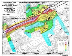 Samples taken
during the main Burn A are shown on Figure 24. Note that there are now three
clearly expressed seepages along the strike of the coal seam outcrop. These
three seepage spots represent the main vertical leakage conduits. A building
placed over one of these spots could develop hazardous concentrations of gases
within the building and in fact over 1000 ppmv of carbon monoxide was found in
the production lab trailer during Burn I in 1979. This required personnel to
wear gas masks to operate their monitoring equipment and greatly increased the
interest in having a better monitoring system for Burn II.
Samples taken
during the main Burn A are shown on Figure 24. Note that there are now three
clearly expressed seepages along the strike of the coal seam outcrop. These
three seepage spots represent the main vertical leakage conduits. A building
placed over one of these spots could develop hazardous concentrations of gases
within the building and in fact over 1000 ppmv of carbon monoxide was found in
the production lab trailer during Burn I in 1979. This required personnel to
wear gas masks to operate their monitoring equipment and greatly increased the
interest in having a better monitoring system for Burn II.
 Contoured
magnitude maps of propane, carbon monoxide, carbon dioxide, and hydrogen for
the four time periods discussed above are available (Jones and Thune, 1982).
In the area surrounding Burn I, relatively high values of each of these gases
were still present in the near surface prior to Burn II. Detailed examination
of these maps together with the geologic map indicates that most of the higher
concentrations are found stratigraphically above the gasified "G"
coal. Comparing the pre-burn maps with the facility installation map shows
that higher values are found around or near the principal injection and product
wells. This clustering may be due to leakage resulting from poor cement jobs
on the wells.
Contoured
magnitude maps of propane, carbon monoxide, carbon dioxide, and hydrogen for
the four time periods discussed above are available (Jones and Thune, 1982).
In the area surrounding Burn I, relatively high values of each of these gases
were still present in the near surface prior to Burn II. Detailed examination
of these maps together with the geologic map indicates that most of the higher
concentrations are found stratigraphically above the gasified "G"
coal. Comparing the pre-burn maps with the facility installation map shows
that higher values are found around or near the principal injection and product
wells. This clustering may be due to leakage resulting from poor cement jobs
on the wells.
Of special interest is the obvious "streaming" in a northerly direction along the strike of, and mainly within, the friable sandstones overlying the "G" coal. This "streaming" within this horizon is a well developed feature recognizable on all of the geochemical maps. On the methane pressure period map (Figure 23) the high values are mainly restricted to the area surrounding Burn I. Pressuring of the "G" coal was done through one of the Burn II injection wells. Increases in methane values largely took place in the area surrounding Burn I, and to a lesser extent to the north, but again mainly in the overlying sandstones. This would indicate that there is a major migration path probably associated with the well developed fracture pattern contained within the sandstones. Of special interest is the anomaly that appears along the strike of the coal outcrop, at the northern boundary of the facility. The anomaly occurred within hours of the very large magnitude anomaly that occurred directly updip from the retort and is interpreted to represent pressure driven migration along fractures. During Burn I, product gases preferentially migrated updip to the east and then along strike and were still present in those rocks nearly a year after shutdown of that burn. While diffusion through the sandstone overlying the "G" coal cannot be ruled out, it appears that migration northward along the well developed dominant "strike" joint set and upward along the subordinate cross-joint set provides the major migration paths from the product source.
The northerly trending "streaming" through the sandstone overlying the “G” coal is obvious, and a study of the rate at which the high methane values developed at the northernmost monitoring points suggests that well developed jointing may have provided the major avenues for product gas migration from the gasification retort. On these maps (Figures 24 and 25) the slight increase in methane values vertically over the retort as compared to the increases seen along the outcrop of the sandstone overlying the "G" coal strengthens the argument that diffusion as a transport mechanism is of only minor importance as compared to migration associated with fracturing. This is particularly so because of the apparent lack of "streaming" of the leaked products to the north along the beds vertically over the burn.
 After the burn
was well established and the working pressures on the gasification system could
be lowered, there appeared to be a slight decline in the magnitudes of leaked
gases in the near surface. The lack of a clear-cut decline after burn shutdown
can be explained by the fact that the affected sediments carrying the product
gases were already near saturation. When the pressures on the retort were
removed, the drive "forcing" the gases to the surface no longer
existed, and the gases remaining within the reservoir continued to migrate, but
at a slower rate than when under pressure. The presence of relatively high
values of product hydrocarbon gases remain in the area surrounding Burn I
nearly 1 year after its shutdown. Once the retort was depressured and filled
with water the seepage magnitudes, decreased rapidly, however they were still
measurable one year after Burn II, and as noted on Figure 22, gases were still
present 2 years after Burn I. Unfortunately we did not have any monitoring
wells during Burn I, so we cannot estimate how much the soil gas values have
decreased following Burn I.
After the burn
was well established and the working pressures on the gasification system could
be lowered, there appeared to be a slight decline in the magnitudes of leaked
gases in the near surface. The lack of a clear-cut decline after burn shutdown
can be explained by the fact that the affected sediments carrying the product
gases were already near saturation. When the pressures on the retort were
removed, the drive "forcing" the gases to the surface no longer
existed, and the gases remaining within the reservoir continued to migrate, but
at a slower rate than when under pressure. The presence of relatively high
values of product hydrocarbon gases remain in the area surrounding Burn I
nearly 1 year after its shutdown. Once the retort was depressured and filled
with water the seepage magnitudes, decreased rapidly, however they were still
measurable one year after Burn II, and as noted on Figure 22, gases were still
present 2 years after Burn I. Unfortunately we did not have any monitoring
wells during Burn I, so we cannot estimate how much the soil gas values have
decreased following Burn I.
Previous exploration surveys completed over the Hartzog Draw field in 1976 had shown that seeps decreased in magnitude as the subsurface reservoir pressures were reduced. This was hard to prove by conducting a second survey over a producing field because environmental changes such as rainfall, barometric pressure, etc, could have affected the data. However, the data taken over the coal burn project indicate a recognizable surface response occurred 3-5 days after changes in the burn retort pressures. In 1980 these observations were supplemented by other surveys over gas storage fields that provided conclusive evidence that seep magnitudes would in fact respond quickly to venting of the gas pressures within the subsurface reservoirs.
Salt Dome Storage Cavern Monitoring
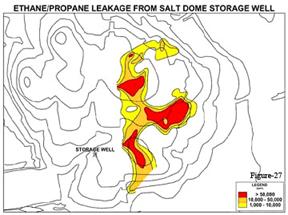 The Barbers Hill Salt Dome
Cavern Leak
The Barbers Hill Salt Dome
Cavern Leak
At the Barbers Hill salt dome, a storage cavern well lost its product (an ethane/propane mix) through a corrosion hole in the casing within the cap rock at about 600 feet (Jones, 1984, Pirkle, 1986,Pirkle and Price, 1986, Jones and Burtell, 1994). Estimates of total product lost were in the range of 109 ft3. The escaping product bypassed several sand units above the caprock, presumably by following fault and fracture conduits or an abandoned well. The lost product migrated updip toward the top of the dome with major accumulations in sands at the 200 foot level. From there, migration to the surface continued with widespread gas presence found in the near surface 30 foot water sand at lateral distances of > 3000 feet.
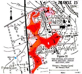 A surface soil
gas survey (see Figures 27 and 28) was successfully used to map the lost
product and direct a mitigation effort. The soil gas contours overlayed on a
contour map of the cap rock are shown in Figure 27 and overlayed on a culture
base in Figure 28. Approximately 500 monitoring wells were installed on 50 to
100 foot centers to a depth of 30 feet to encounter the gas in the 30 foot
water sand both on the facility property and in the town of Mont Belvieu.
Relief wells for the major accumulation at 200 feet were drilled along a NW-SE
alignment, presumably a fault zone, defined by aerial photography and soil gas
data. Soil gas concentrations at 30 feet were higher by a factor of 500 - 1000
within this zone. The produced product was flared in order to release the
subsurface pressure. The first well, after an initial blow out, produced at a
rate of 10 mmcfd for several days. More than thirty relief wells were drilled
over the anomalous area in order to relieve the subsurface pressure.
A surface soil
gas survey (see Figures 27 and 28) was successfully used to map the lost
product and direct a mitigation effort. The soil gas contours overlayed on a
contour map of the cap rock are shown in Figure 27 and overlayed on a culture
base in Figure 28. Approximately 500 monitoring wells were installed on 50 to
100 foot centers to a depth of 30 feet to encounter the gas in the 30 foot
water sand both on the facility property and in the town of Mont Belvieu.
Relief wells for the major accumulation at 200 feet were drilled along a NW-SE
alignment, presumably a fault zone, defined by aerial photography and soil gas
data. Soil gas concentrations at 30 feet were higher by a factor of 500 - 1000
within this zone. The produced product was flared in order to release the
subsurface pressure. The first well, after an initial blow out, produced at a
rate of 10 mmcfd for several days. More than thirty relief wells were drilled
over the anomalous area in order to relieve the subsurface pressure.
The product lost was an ethane-propane mix which has a unique signature as compared to the normal hydrocarbon products originally found in the natural reservoirs associated with this salt dome. In some of the surveyed areas, the contaminant found was mainly propylene. This was traced to an earlier reported spill by another operator on the dome, as documented from the historical records, which was previously thought to have no known surface expression.
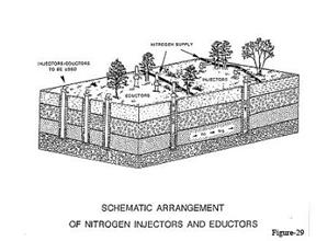 The cleanup
operation, shown in schematic on Figure 29, was facilitated by vapor extraction
of the 30 foot water sand using the geochemical monitor wells. Vacuum was
provided by installing a venturi tube on the top of the well casing. Nitrogen
was run through the venturi tube to produce a small vacuum on the formation.
To aid in the process, nitrogen was injected at monitor wells about 50 feet
away, essentially giving a push to the hydrocarbon plume. In order to follow
this N2 flood process, Gulf converted helium/hydrogen gas
chromatographs, typically used for exploration seep detection, to
nitrogen/oxygen detectors.
The cleanup
operation, shown in schematic on Figure 29, was facilitated by vapor extraction
of the 30 foot water sand using the geochemical monitor wells. Vacuum was
provided by installing a venturi tube on the top of the well casing. Nitrogen
was run through the venturi tube to produce a small vacuum on the formation.
To aid in the process, nitrogen was injected at monitor wells about 50 feet
away, essentially giving a push to the hydrocarbon plume. In order to follow
this N2 flood process, Gulf converted helium/hydrogen gas
chromatographs, typically used for exploration seep detection, to
nitrogen/oxygen detectors.
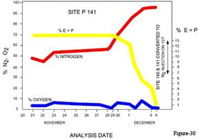 Typical response
curves illustrating the advance of the nitrogen front and cleanup of the E/P
product mix are shown in Figure 30. This illustrates the rapidity with which
the nitrogen front passed through the 30 foot aquifer in this area. The
nitrogen flood pushed the lost product laterally back onto Gulf's property
through the shallow 30 foot sand after the pressure was relieved in the deep
200 foot sand, thus cleaning up and preventing any recharge to the local
residences.
Typical response
curves illustrating the advance of the nitrogen front and cleanup of the E/P
product mix are shown in Figure 30. This illustrates the rapidity with which
the nitrogen front passed through the 30 foot aquifer in this area. The
nitrogen flood pushed the lost product laterally back onto Gulf's property
through the shallow 30 foot sand after the pressure was relieved in the deep
200 foot sand, thus cleaning up and preventing any recharge to the local
residences.
The time rate of cleanup response over the entire area turned out to be useful for illustrating the variation in lithology and permeability, neither of which were uniform, and clearly demonstrated a significant influence on lateral gas migration. In some cases, the permeability was so low that 15 lbs of nitrogen pressure at 30 feet was not sufficient to push the gas 50 feet laterally over to the next vapor extraction station; yet, if a bucket of water were poured on the ground near the injection site, the ground would froth and bubble from the nitrogen that was escaping vertically through 30 feet of Beaumont clay. This vertical nitrogen leakage occurred in spite of the fact that the nitrogen would not travel laterally to the next eductor site. It appeared that most of these spots had a better association with deeper vertical migration pathways rather than from lateral migration through the 30 foot sand.
A Mississippi Salt Dome Cavern Leak
A second salt dome example (Pirkle, 1986, Pirkle and Price, 1986) comes from a small dome in Mississippi which had 4 caverns which stored natural gas. The initial survey was commissioned to investigate suspected leaks in one of the 4 storage caverns.
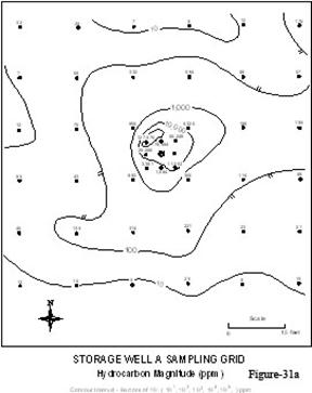
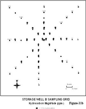 A grid of samples on a 15 foot
spacing were taken at a depth of 3 feet as shown in Figure 31a. Anomalous
concentrations of hydrocarbons are contoured,, which have a natural gas
composition and confirm the suspected leak. The well was shut in and repairs
undertaken. While present at the site, samples were taken near the other three
storage caverns to check for presence of natural gas product. At two of the
storage wells no evidence of leakage was found, however at one well a very
large pattern of hydrocarbon product at combustible concentrations was found.
Data from this well are shown in Figure 31b. At sites marked with an asterisk,
soil gas concentrations are > 15%. This well was also emptied and shut down
for repairs.
A grid of samples on a 15 foot
spacing were taken at a depth of 3 feet as shown in Figure 31a. Anomalous
concentrations of hydrocarbons are contoured,, which have a natural gas
composition and confirm the suspected leak. The well was shut in and repairs
undertaken. While present at the site, samples were taken near the other three
storage caverns to check for presence of natural gas product. At two of the
storage wells no evidence of leakage was found, however at one well a very
large pattern of hydrocarbon product at combustible concentrations was found.
Data from this well are shown in Figure 31b. At sites marked with an asterisk,
soil gas concentrations are > 15%. This well was also emptied and shut down
for repairs.
These and other examples indicate the potential for wells to leak around their casings, usually as the result of poor cement jobs at the time of casing installation. This may be particularly significant in the case of carbon sequestration because of the potential presence over most formerly productive fields of numerous plugged and abandoned wells. In the case of these storage wells the potential conduit is for the most part limited to poor cement jobs related to casing installation. In the case of plugged and abandoned (P&A) wells over a petroleum reservoir, the potential for leakage is not only related to casing cement, but could also result from improper P&A procedures as well. That is to say that these wells could be essentially open to the surface from some point at depth.
A Mined Gas Storage Cavern Leak
Another excellent opportunity resulted from a study conducted over a 200 foot deep propane storage cavern (Jones, 1984, Pirkle, 1986, Pirkle and Price, 1986, Jones and Burtell, 1994). The immediate objective was to determine the leakage rates and to test whether or not ongoing remedial efforts to repair the leaks around the central shaft were successful. Although this was a fairly small facility, 455 geochemical measuring stations were installed to a depth of 20 feet using PVC pipe placed on 10 foot centers. Figure 32 shows the propane collected over the cavern plotted on a log scale.
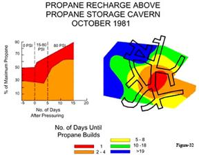 As attempts were
made to repair the leaks in the central shaft, the cavern pressure was
decreased to ambient levels as repairs were made, and then repressured allowing
the recharge leakage rate from the cavern to be remeasured. Upon recharging
the cavern, the time it took for the propane gas to reestablish its maximum
leakage values at the surface was measured. As shown by Figure 32, following
the recharge of the cavern with propane to its original pressure, a value of
over 90% of the original soil gas propane concentration was observed within the
observation test holes within 15 days. Most of the leakage came from around
the central shaft. However, it was expected that must be a large propane
background in the soil since the storage site had been known to leak for over
20 years. This propane background made it difficult to be sure the product
reappearing at the surface came directly out of the reservoir during the
sampling time period.
As attempts were
made to repair the leaks in the central shaft, the cavern pressure was
decreased to ambient levels as repairs were made, and then repressured allowing
the recharge leakage rate from the cavern to be remeasured. Upon recharging
the cavern, the time it took for the propane gas to reestablish its maximum
leakage values at the surface was measured. As shown by Figure 32, following
the recharge of the cavern with propane to its original pressure, a value of
over 90% of the original soil gas propane concentration was observed within the
observation test holes within 15 days. Most of the leakage came from around
the central shaft. However, it was expected that must be a large propane
background in the soil since the storage site had been known to leak for over
20 years. This propane background made it difficult to be sure the product
reappearing at the surface came directly out of the reservoir during the
sampling time period.
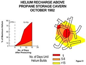 To solve this
problem and provide a more definitive test, helium was injected into the cavern
at a concentration of about 600 ppm. Results showed that in 15 days, not only
had the product moved, but as shown in Figure 33, helium was also detected at
the surface. Helium injection not only showed the leakage around the central
cavern, but also found a leak at the end of one of the drifts that would have
been missed looking only at propane. The amount of helium used for this test
was not enough to damage the product for sale, and yet still gave more than
adequate sample for analysis. This helium injection test proved that migration
was quite rapid, further confirming the results from the underground coal
gasification reactor, where migration times of from 3 to 5 days at depths of up
to 600 to 1000 feet were observed for changes of gas concentrations in the
reservoir or cavern to be expressed at the surface. This means migration does
not follow a diffusion model, but is driven by pressure, with migration driven
along fault and fracture patterns and joints. Results of the studies of
Underground Gas Storage Facilities were presented at several professional
meetings (Pirkle, 1986; Pirkle & Price, 1986)).
To solve this
problem and provide a more definitive test, helium was injected into the cavern
at a concentration of about 600 ppm. Results showed that in 15 days, not only
had the product moved, but as shown in Figure 33, helium was also detected at
the surface. Helium injection not only showed the leakage around the central
cavern, but also found a leak at the end of one of the drifts that would have
been missed looking only at propane. The amount of helium used for this test
was not enough to damage the product for sale, and yet still gave more than
adequate sample for analysis. This helium injection test proved that migration
was quite rapid, further confirming the results from the underground coal
gasification reactor, where migration times of from 3 to 5 days at depths of up
to 600 to 1000 feet were observed for changes of gas concentrations in the
reservoir or cavern to be expressed at the surface. This means migration does
not follow a diffusion model, but is driven by pressure, with migration driven
along fault and fracture patterns and joints. Results of the studies of
Underground Gas Storage Facilities were presented at several professional
meetings (Pirkle, 1986; Pirkle & Price, 1986)).
Barometric Pressure and its Relationship to Gas Flux
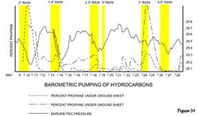 Mined Gas Cavern Example
Our early investigations into the relationship of barometric pressure and gas flux were carried out at an underground storage cavern (Pirkle, 1986, Pirkle and Price, 1986, Jones and Burtell, 1994). Plastic ground sheets about 5 feet square were installed directly over known leakage areas to measure the gas flux related to meteorological and barometric changes. The data, including rainfall amounts and timing, are shown on Figure 34. A very large gas flux is shown by the dashed line during the early days of the measurements. This flux is no doubt associated with the associated rapid decrease in barometric pressure and perhaps with the rainfall event, however in these early experiments, the groundsheet integrity was often affected adversely by rainfall and the correlation over time suffered as a result. Improvements in groundsheet construction, as shown in the following example, yielded much more predictable gas flux data.
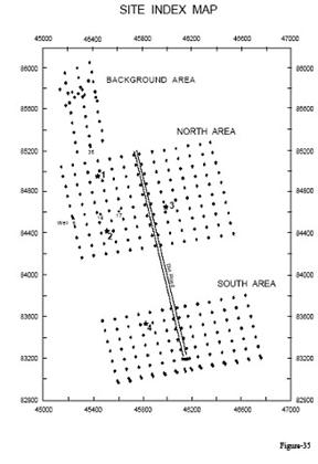 The Savannah River
Site Sanitary Landfill Example
The Savannah River
Site Sanitary Landfill Example
The following example (Pirkle, et. al., 1992) is from a shallow landfill at the Savannah River Site near Aiken, SC. The landfill established in 1974 covers an area of about 70 acres. Burial has been in excavated earthen trenches and the known disposal includes paper, plastic, construction debris, solvent rags, metal debris and carcasses.
A soil gas survey was carried out in December 1990 with an objective to determine the presence and extent of volatile contaminants in near surface soil gases. A sample grid on 100 foot centers consisting of 288 sample locations was established as shown on Figure 35. Samples were taken from a nominal depth of 3 feet. Species monitored were the light hydrocarbons C1 - C4; gasoline range normal paraffins and aromatics, C5 - C10; and selected chlorinated organics. Low levels of volatile organics compounds including trichloroethylene, tetrachloroethylene, and 1,1,1-trichloroethane had been reported at a groundwater monitoring well at the site.
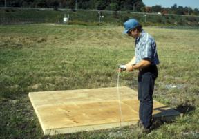 The results of
the soil gas survey confirmed that a variety of common petroleum based fluids
and chlorinated solvents had been a part of the materials buried at the
landfill. Methane, generated from the biological degradation of cellulose and
other organic materials was found in concentrations ranging up to 65% by
volume. These observations of large concentrations of volatile species,
including methane, led to a survey to determine if these gases could move
through the nominal 3 foot soil cover over the trenches and into the
atmosphere. To accomplish this, 4 groundsheets (8 x 8 feet square) as shown in
Figure 36 were placed at selected locations at the landfill based on methane
concentrations determined in the soil gas survey.
The results of
the soil gas survey confirmed that a variety of common petroleum based fluids
and chlorinated solvents had been a part of the materials buried at the
landfill. Methane, generated from the biological degradation of cellulose and
other organic materials was found in concentrations ranging up to 65% by
volume. These observations of large concentrations of volatile species,
including methane, led to a survey to determine if these gases could move
through the nominal 3 foot soil cover over the trenches and into the
atmosphere. To accomplish this, 4 groundsheets (8 x 8 feet square) as shown in
Figure 36 were placed at selected locations at the landfill based on methane
concentrations determined in the soil gas survey.
Samples were taken from underneath each of the four groundsheets every four hours for a period of two weeks. Each sample was analyzed using gas chromatography for the C1 – C4 hydrocarbons. Selected samples were analyzed for the volatile organics found in the soil gas survey.
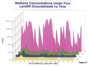 Methane
concentrations from all samples taken from under each of the four groundsheets
are shown on Figure 37. Concentrations under each groundsheet were observed to
vary greatly over the two weeks of observation. Concentrations observed under
groundsheet #2 are much larger than under groundsheets 1, 3 or 4. Careful
study of Figure 37 reveals that despite the differences in magnitude, the
variation of methane concentrations under all 4 groundsheets are approximately
in phase. This would be expected if these variations in concentration resulted
from a single driving force such as barometric pumping.
Methane
concentrations from all samples taken from under each of the four groundsheets
are shown on Figure 37. Concentrations under each groundsheet were observed to
vary greatly over the two weeks of observation. Concentrations observed under
groundsheet #2 are much larger than under groundsheets 1, 3 or 4. Careful
study of Figure 37 reveals that despite the differences in magnitude, the
variation of methane concentrations under all 4 groundsheets are approximately
in phase. This would be expected if these variations in concentration resulted
from a single driving force such as barometric pumping.
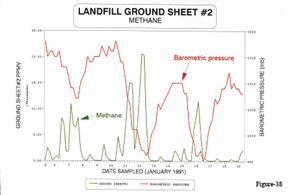 Methane under
groundsheet #2 and barometric pressure are shown as a function of time on
Figure 38. Methane concentrations under this groundsheet increase rapidly
during periods of falling barometric pressure. Close study of the data reveals
that even periods of stable pressure in an overall falling pressure regime are
sufficient to cause cessation of the methane flux.
Methane under
groundsheet #2 and barometric pressure are shown as a function of time on
Figure 38. Methane concentrations under this groundsheet increase rapidly
during periods of falling barometric pressure. Close study of the data reveals
that even periods of stable pressure in an overall falling pressure regime are
sufficient to cause cessation of the methane flux.
Some variations in the rate of methane flux over the course of these observations may be attributable to changes in soil moisture content as a result of periodic heavy rains during the observation period, similar to observations by McNerney and Buseck 1973. Increases in soil moisture are thought to decrease the permeability of the soil and impede the pressure equilibration which causes the flow of soil gas through the soil/atmosphere boundary.
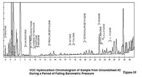 The other light
hydrocarbons exhibited variations similar to methane. The only significant
difference was their much smaller concentration. One sample which corresponded
to a methane maximum under groundsheet #2, was further analyzed for volatile
organics. A chromatogram of that sample, shown in Figure 39, reveals that many
of not all of the complex volatile organic species buried at the landfill
migrate vertically through the soil/atmospheric boundary into the atmosphere.
The flux is maximized during periods of falling barometric pressure and ceases
or is minimized during periods of stable or rising pressure.
The other light
hydrocarbons exhibited variations similar to methane. The only significant
difference was their much smaller concentration. One sample which corresponded
to a methane maximum under groundsheet #2, was further analyzed for volatile
organics. A chromatogram of that sample, shown in Figure 39, reveals that many
of not all of the complex volatile organic species buried at the landfill
migrate vertically through the soil/atmospheric boundary into the atmosphere.
The flux is maximized during periods of falling barometric pressure and ceases
or is minimized during periods of stable or rising pressure.
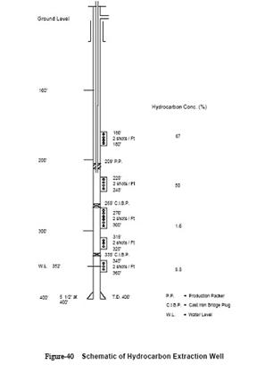 Western Salt Block Cavern
Example
Western Salt Block Cavern
Example
During the assessment and remediation of a subsurface propane release (Pirkle, et. al, 1992), data were gathered which suggested that barometric pumping may be effective to considerable depth. At this site propane had bee released at a depth of approximately 100 feet and had been detected in several strata down to the water table at 350 feet.
Shown in Figure 40, is the schematic of a well drilled to the water table for the purpose of hydrocarbon withdrawal. The well casing was perforated in zones of significant propane concentrations as determined by the analysis of the mud stream during drilling. The largest propane concentrations were found in zones between 160 - 180 feet (Zone 1) & 225 - 245 feet (Zone 2). These zones were isolated from the lower zones by using a bridge plug at 265 feet & were separated from each other using a production packer. Barometric pressure was determined from an onsite recording barometer. Subsurface pressures were determined using two water manometers: the first between the atmosphere & Zone 2; & the second across Zones 1 & 2. Using pressure data from the recording barometer & the pressure differentials from the water manometers, the pressures in both zones were calculated.
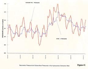 The subsurface
pressure in Zone 2 vs barometric pressure is shown on Figure 41. Careful
examination of these data reveal that even diurnal changes in barometric
pressure at the surface are accompanied by changes in subsurface pressure at
225 – 245 feet, although there is a time lag between the maxima of barometric
and subsurface pressure. The changing subsurface pressures result in vertical
movement of soil gases relative to the perforations in the well.
The subsurface
pressure in Zone 2 vs barometric pressure is shown on Figure 41. Careful
examination of these data reveal that even diurnal changes in barometric
pressure at the surface are accompanied by changes in subsurface pressure at
225 – 245 feet, although there is a time lag between the maxima of barometric
and subsurface pressure. The changing subsurface pressures result in vertical
movement of soil gases relative to the perforations in the well.
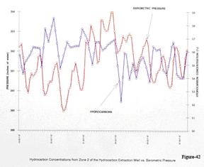 As shown on
Figure 42, this vertical soil gas movement is evidenced by propane
concentrations which change as a function of time similar to changes in diurnal
barometric pressure. The propane concentrations were determined from samples
taken as Zone 2 was continuously pumped. The changes in concentration
apparently result from vertical gradients in propane concentration in the
strata opposite the perforations. Gas pumped through the perforations thus has
differing propane concentrations as the soil gases move vertically in the sediments in response to changes in barometric pressure.
As shown on
Figure 42, this vertical soil gas movement is evidenced by propane
concentrations which change as a function of time similar to changes in diurnal
barometric pressure. The propane concentrations were determined from samples
taken as Zone 2 was continuously pumped. The changes in concentration
apparently result from vertical gradients in propane concentration in the
strata opposite the perforations. Gas pumped through the perforations thus has
differing propane concentrations as the soil gases move vertically in the sediments in response to changes in barometric pressure.
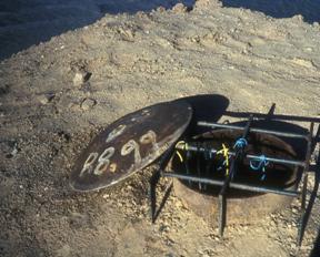 At the site just
discussed, it was also noticed that gas periodically emanated from an open
abandoned water well, shown in Figure 43, about 300 feet from the hydrocarbon
withdrawal well discussed above.
At the site just
discussed, it was also noticed that gas periodically emanated from an open
abandoned water well, shown in Figure 43, about 300 feet from the hydrocarbon
withdrawal well discussed above.
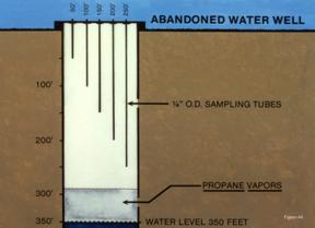 Investigation of
these periodic gas flows was accomplished by installing sampling tubes to
several depths in the well as shown schematically in Figure 44. Samples were
taken from each tube every 4 hours for a period of time and analyzed for the
light hydrocarbons C1 – C4.
Investigation of
these periodic gas flows was accomplished by installing sampling tubes to
several depths in the well as shown schematically in Figure 44. Samples were
taken from each tube every 4 hours for a period of time and analyzed for the
light hydrocarbons C1 – C4.
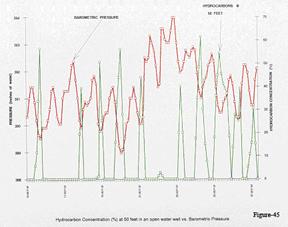 The results are shown on Figures
45 and 46 which show propane concentrations at 50 and 254 feet in the well as a
function of time and barometric pressure. It is apparent that there is a
source of propane at depth which can get into this abandoned well with
concentrations of approximately 50 – 60 % by volume, similar to concentrations
observed in Zones 1 and 2 of the propane withdrawal well. This column of
propane moves from depth in the well to the surface as a result of the normal
diurnal excursions of barometric pressure and is an excellent illustration of
the phenomenon of barometric pumping. In the sedimentary column, the large
movement of gas is impeded, but not stopped by the reduced permeability and
tortuous path introduced by packed sedimentary particles.
The results are shown on Figures
45 and 46 which show propane concentrations at 50 and 254 feet in the well as a
function of time and barometric pressure. It is apparent that there is a
source of propane at depth which can get into this abandoned well with
concentrations of approximately 50 – 60 % by volume, similar to concentrations
observed in Zones 1 and 2 of the propane withdrawal well. This column of
propane moves from depth in the well to the surface as a result of the normal
diurnal excursions of barometric pressure and is an excellent illustration of
the phenomenon of barometric pumping. In the sedimentary column, the large
movement of gas is impeded, but not stopped by the reduced permeability and
tortuous path introduced by packed sedimentary particles.
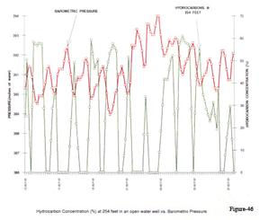
The UCG example discussed above not only showed the strong control that bedding planes could have on migration avenues, but it also showed that the influence of the local fracture system was equally important. As shown in Figures 22-26, three major methane anomalies were observed along the strike of the bedding plane. This indicated the leakage gases did not migrate updip along the bedding plane, and then migrate laterally along the strike of the beds to fill the surface sediments with gas. Instead, the leakage gases came up almost simultaneously within three localized areas, or "hydrocarbon spots". This concept suggests a migration pattern with gases moving along a complex mixture of bedding planes and fracture avenues at depth. The locations of the "hydrocarbon spots" at the surface are controlled by these complex pathways, and as such appear to be somewhat predictable from geologic mapping. This UCG seepage data is an excellent demonstration of a property of hydrocarbon seeps that we have discerned from numerous examples cited here. "Hydrocarbon spots" are connected to sources at depth through migrational conduits which are predetermined at every site by geological conditions. Once defined, these conduits will provide predictable and reliable pathways for all future pressure relief from depth, and their surface manifestation, the “hydrocarbon spots”, can be used to establish a permanent monitoring system.
The term "hydrocarbon spots" was coined from previous earthquake prediction studies carried out by the Japanese. Two landmark publications by Wakita et al., (Science, 1978) have indicated that both helium and hydrogen are observed in anomalous quantities along faults. In 1978 helium was observed to be as large as 350 ppm within a nitrogen vent on the Matsushiro fault swarm. The authors proposed to call these anomalous areas "Helium Spots" because the helium leakage was not homogeneous throughout the fault zone. These unevenly distributed helium spots were reported to occupy areas of about 30 x 50 meters. Extensive experience in soil gas prospecting by Gulf has revealed that all soil gas anomalies occur in such spots. This is obvious because the migration of gases is dominated by faults and fractures, either on the macro or micro scale. A second paper, by Wakita, (Science, 1980), reported 70 measurements for hydrogen in the Yamasaki fault zone. These measurements, made in 0.5 to 1 meter deep holes, reported hydrogen anomalies ranging from 2 to 30,000 ppm H2 in the fault zone, with background values of 0.5 ppm observed outside the influence of the fault. The authors postulated that hydrogen was formed by the reaction between groundwater and fresh rock surfaces formed by fault movement. Clearly, additional information on gas leakage patterns in the earth could be gained from the extensive literature on gas flux related to earthquakes.
Deep Mobile Gases and Their Relation to Earthquakes
Further examinations of the published literature, coupled with extensive field applications by Gulf Research scientists indicated that large volumes of diverse gases continually escape from the earth's crust into the atmosphere. Areas of especially high activity are reported to be related to zones of deep tectonic fracturing and the accompanying jointing in which mineralization is sometimes located. Typical deep gases are CO2, N2, CH4, H2, He, Ar, Rn, Hg, SO2, COS and H2S. The major components are CO2, N2, CH4, and H2; with the remainder of this list generally found as minor or trace components. The isotopic composition of hydrogen, carbon, and oxygen, are reported to have considerable potential for helping to define the sources of these gases. According to published literature, the magnitudes of deep gas anomalies are governed strongly by tectonic and magmatic activity, thus stronger patterns are encountered in seismically active areas of late orogenic activity. Accordingly, the weaker patterns are observed in platform and shield areas that are relatively quiescent; that is in consolidated blocks of the earth's crust. These observations had obviously been confirmed by our previous experience.
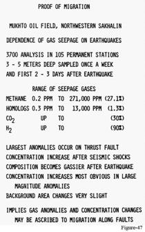
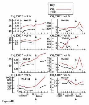
Numerous published examples of gas flux related to earthquakes have been reported, Barsukov (1979), Borodzich (1979), Elinson, et al. (1971), Eremeev (1972), Fursov (1968), Pirkle and Jones (1983), Kartsev (1959), King (1980), Mamyrin (1979), Melvin (1978, 1981), Mooney (1982), Ovchinnikov (1972), Reimer (1980), Shapiro, et al. (1981, 1982), Sokolov (1971), Wakita, et al. (1978, 1980) and Zorkin (1977), to name only a few papers.
One particularly impressive study by the Soviets showed that the magnitude of soil gas values on faults increase dramatically shortly after an earthquake in which fault movement was involved (Zorkin, et al., 1977). An extensive study, involving 105 observation wells 3 to 5 meters deep, was set up over the Mukhto Oil Field on northeastern Sakhalin Island. Thirty-seven hundred samples were collected and analyzed over a four month period with the most active wells sampled daily. Figures 47 and 48 from this study provide impressive evidence for the tectonic relationship of this leakage gas flux. This study leaves no doubt that faults and fractures provide the main control on the migration of gases from the subsurface.
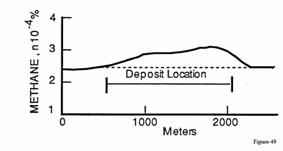
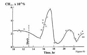
Many intriguing examples (see Figures 49 and 50) have been published by Antropov, et al. (1981) of atmospheric methane flux related to petroleum deposits, and seismic shock. These measurements were made with adsorption type gas lasers. Two types have been described: one measures the sample in an adsorption tube (Iskatel-2), while the other (Luch) measures the specific gas adsorption along an optical path. One makes point measurements while the other averages the adsorption over a long path length (1-100 meters).
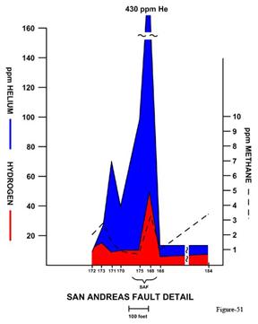 San Andreas Fault Example
Geochemical monitoring related to earthquake activity was not widely practiced in the US where most efforts were geophysical until about 1975. Programs using radon began about 1975 at Cal-Tech at about the same time that Gulf Research scientists first made measurements on light hydrocarbons, helium, and hydrogen on the San Andreas Fault in the Cholame Valley in California (Jones and Drozd, 1983). An early published example, shown in Figure 51, confirmed helium is a deep basement, or tectonic indicator which is commonly independent of oil and gas deposits. At Cholame, where this profile is located, the fault moved in 1857, 1906, 1922 and most recently in 1966. Figure 52 shows two pictures taken immediately after the 1966 earthquake, the first on July 22nd when the offset was only two inches, and then again 12 days later on August 4th when the highway offset had increased to five inches (Iacopi, 1976).
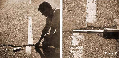
After having documented both natural micro-seeps and manmade macro-seeps over individual commercial fields and underground storage reservoirs, it became apparent that the next step to take was to determine the natural variations that occurred by acquiring gas flux data from an active fault. The level of seismic activity associated with the San Andreas Fault in California makes this geologic province an obvious choice. In order to accomplish this objective, Gulf embarked on a corporate level research project entitled "Gas Flux Related to Earth Motions" in 1981. Evaluation of the known earthquake prediction programs at the USGS and various other universities revealed that the Kellogg Radiation Laboratory at Caltech in Pasadena, CA had the only computerized system which could provide automatic data collection of a series of geochemical variables.
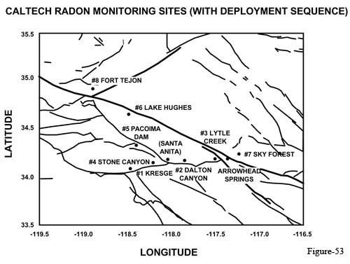 Caltech
scientists had established a network of automated Radon-Thoron monitors
operated by a microcomputer so data could be collected almost continuously
(every eight hours), stored onsite in the computer memory and then transmitted
back to the central laboratory at Caltech over regular telephone lines on
command from a remote computer (Shapiro et al., 1981). Since Gulf's research
objective was to map short-term flux changes, this computer link was an
essential requirement. As shown in Figure 53, Caltech's operating stations
were located at Fort Tejon, Lake Hughes, Pasadena, Santa Anita, Stone Canyon
Reservoir, Big Dalton Canyon north of Glendora, Lyle Creek, Sky Forest in the
San Bernardino Mountains, and at Pacoima Dam, where Gulf was included in the Caltech
program.
Caltech
scientists had established a network of automated Radon-Thoron monitors
operated by a microcomputer so data could be collected almost continuously
(every eight hours), stored onsite in the computer memory and then transmitted
back to the central laboratory at Caltech over regular telephone lines on
command from a remote computer (Shapiro et al., 1981). Since Gulf's research
objective was to map short-term flux changes, this computer link was an
essential requirement. As shown in Figure 53, Caltech's operating stations
were located at Fort Tejon, Lake Hughes, Pasadena, Santa Anita, Stone Canyon
Reservoir, Big Dalton Canyon north of Glendora, Lyle Creek, Sky Forest in the
San Bernardino Mountains, and at Pacoima Dam, where Gulf was included in the Caltech
program.
The Pacoima Dam Example
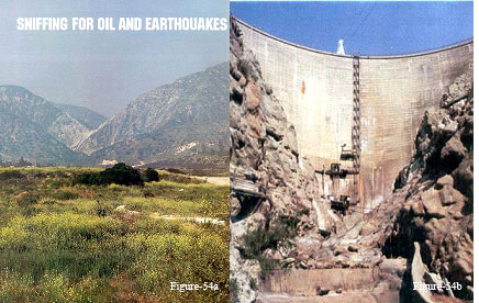
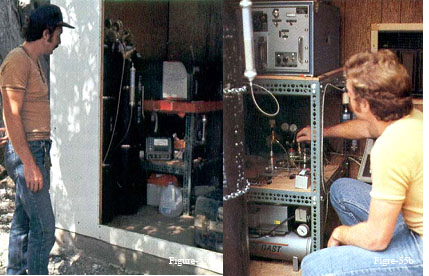
Pacoima Dam was chosen as a site by Caltech scientists because they anticipated micro-seismic activity might be generated by mass loading and unloading within this very steep and fractured valley. Initial measurements made by Gulf at Pacoima Dam indicated that hydrocarbons were of very low concentrations, so Gulf chose to set up this station with a helium-hydrogen gas chromatograph.
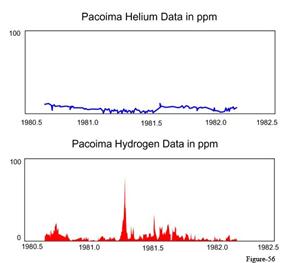 A view of the dam and its
fractured rock walls is shown in Figure 54a & 54b and a close-up view,
which includes the geochemical hut, is shown in Figure 55a & 55b. Shortly
after the gas chromatograph was functioning, a strong hydrogen flux of 75 ppm
was measured in April of 1981, just before a 5.6 magnitude earthquake occurred
near Westmoreland, California. This H2 anomaly lasted nearly three
weeks and peaked sharply at about 75 ppm, as shown in Figure 56. This classic
response provided considerable encouragement to the joint Gulf/Caltech program.
A view of the dam and its
fractured rock walls is shown in Figure 54a & 54b and a close-up view,
which includes the geochemical hut, is shown in Figure 55a & 55b. Shortly
after the gas chromatograph was functioning, a strong hydrogen flux of 75 ppm
was measured in April of 1981, just before a 5.6 magnitude earthquake occurred
near Westmoreland, California. This H2 anomaly lasted nearly three
weeks and peaked sharply at about 75 ppm, as shown in Figure 56. This classic
response provided considerable encouragement to the joint Gulf/Caltech program.
Previous experience in using carbon dioxide to map soil gas anomalies encouraged Gulf to introduce instruments for measuring carbon dioxide at several of the established Caltech stations, such as that shown at Lake Hughes in Figure 53. Within a short time, results from the Lake Hughes station showed the presence of correlated radon and carbon dioxide anomalies. It appeared carbon dioxide reached saturation levels in the water and then served as a carrier for the radon (Shapiro et al., 1982). Although not an earth shaking result (no pun intended), each improvement in measuring and relating the natural gases emanating from these stations increased the possibility of producing interpretable data.
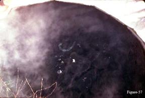 Arrowhead Hot Springs
Example
Arrowhead Hot Springs
Example
Earth gas monitoring studies for possible fluid phase precursors to earthquakes by Scripps Institute of Oceanography also began in 1975 with sampling at Arrowhead Hot Springs (Figure 57) (Jones and Burtell, 1987, Burtell, 1989, Jones and Burtell, 1994). Grab samples of spring gases were collected at one month intervals at the concreted hot spring and analyzed for dissolved radon, helium, nitrogen, temperature, and conductivity. Beginning in 1977, methane was also measured in each sample. Results from these compiled data reflected a variety of short term variations in measured gas content for comparison with seismic events along the San Andreas fault in southern California. The most significant correlation identified was a large increase in measured gases (radon, helium, nitrogen, and methane) in 1979 before the Big Bear earthquake with a magnitude of 4.8 (Craig et al., 1980). This significant increase has been interpreted as the result of an increase in the deep gas component dissolving into hot springs waters. The success of the Scripps' grab sampling program suggested this location would provide even more valuable data for earthquake prediction studies with onsite computer controlled continuous monitoring of gases.
Preliminary gas monitoring by the Gulf/Caltech team at Arrowhead Hot Springs began in early 1981 by collecting gas bubbles with a funnel and gas cylinder. Samples were analyzed for methane, ethane, propane, iso-butane, normal butane, ethylene, propylene, helium and hydrogen by gas chromatography.
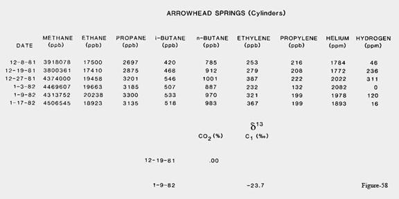
The initial results, shown in Figure 58, indicated the hot springs gases contained 3,918 ppmv of methane, 17.5 ppmv of ethane and 1780 ppmv of helium. The overall high magnitude of measured gases observed upon continued sampling suggested the location was ideal for continuous gas emission monitoring and inclusion into the Caltech/Gulf Research earth gas research programs. A variety of sample collection and analysis methods were employed during sampling at Arrowhead Hot Springs, including a cross check analysis by Dr. John Welham of Scripps as shown in Figure 59. Based on these early results, it was clear Arrowhead was the type of active seepage site Gulf scientists wanted to sample and to include in the Caltech earthquake prediction program.
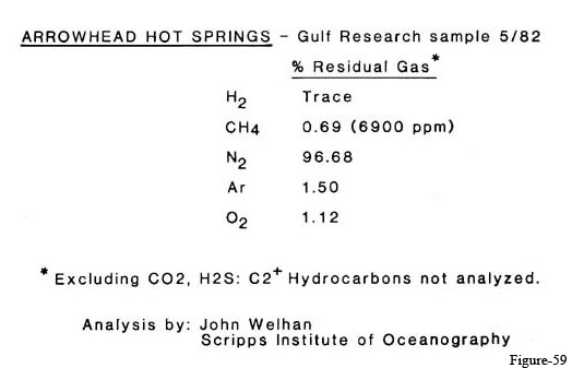
A more detailed description of the geology at Arrowhead Hot Springs is available in Burtell, Jones and Anderson, 1987, Burtell (1989) and in Jones and Burtell (1996). A gas collection system was set up at Arrowhead and semi-continuous gas data collected from Dec. 1981 to Dec. 1982. This included the measurement of light C1- C4 hydrocarbon gases, helium, hydrogen CO2, radon and mercury plus carbon 12/13 isotopes on the methane and helium 3/4 isotopes. Plots of the methane, propane, propane/methane ratio and the helium concentrations versus time are shown by Figures 60, 61, 62 and 63.
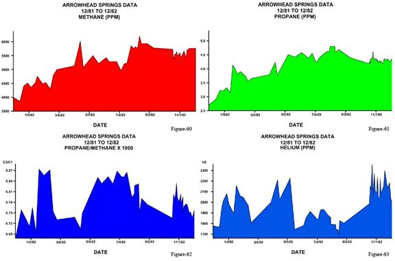
Significant magnitude and compositional changes occurred over the monitoring period. There was a steady rise in methane from 3918 in 1981 to 6000 ppmv by 12/2/82. Helium magnitudes, over this time period, appeared to fluctuate independently of the light hydrocarbon gases, suggesting an independent source for the helium. Overall helium magnitudes ranged between 1700 and 2350 ppmv as free gases from the spring reflected a very concentrated source of helium (over 350 times atmospheric levels). Although the initial Scripps' data suggested a positive correlation between methane and helium for the 1979 Big Bear Earthquake, this more detailed analysis showed this correlation was much more complex and that helium may be affected by different geologic and tectonic events than methane.
The origin of the measured helium appeared to be primarily of crustal radioactive decay, with minor input from mantle sources. Methane and the other light hydrocarbons have a very mature sedimentary signature, with a methane carbon 13/12 isotope ratio of -23.7 parts per thousand relative to PDB. This is the most mature methane ever measured by Gulf Research, including many 30,000 foot deep west Texas gases from the Gomez Gas Field. This mature organic hydrocarbon gas strongly suggests that sedimentary rocks are present below crystalline and metamorphic rocks of the San Bernardino Mountains. The possibility is strongly supported by recent geologic research which indicates low angle thrust faults of Laramide to Tertiary age in the Mojave desert in the east. Tectonic activity may have thrust the San Bernardino Mountain block over sedimentary formations which now lie below the San Bernardino Mountains. Subsequent burial and maturation of sedimentary source rock may have produced significant quantities of hydrocarbons.
This project began as a spin-off of a joint Gulf Research-Caltech deep fault gas flux monitoring program to assist Caltech in the development of vapor phase earthquake prediction techniques and to improve Gulf's understanding of gas migration mechanisms. The resultant investigations have tested various assumptions and theories about deep fault and fracture system gas emanations and their expression at near- surface sampling sites. Each phase of the program was completed to help develop geochemical sampling techniques, start a data base for future programs, and as an aid for the evaluation of potential earthquake prediction sites.
This program focused mainly on the study of a single hot spring site in an attempt to relate gas emissions to earthquakes. Light hydrocarbons, helium, radon, hydrogen, carbon dioxide, and carbon monoxide were monitored for magnitude and compositional changes and correlation with earthquake occurrences. Although no clear earthquake related events were identified, significant gas magnitude and compositional changes were recorded. Regional stress variations were interpreted as the most probable cause for the recorded changes in gas flux at this site. Plans for additional sites and longer term monitoring were made by Gulf and Caltech scientists and are highly recommended for future research. Industry downsizings and takeovers prevented the final implementation of these research plans.
For the first time, we had gas flux data on a deep active fault that provided us with actual variations in concentration that are generated by earth tectonics, where the sampling methods, temperatures and other meteorological changes have no effect. The Arrowhead Springs data exhibited changes in the propane/methane ratio, indicating that stress changes deep within the earth were causing releases of methane and propane and their travel time from the release point to the surface hot spring was likely different enough to cause the change in composition, much like the Russians noted over the Mukhto Oil Field on Sakhalin Island.
One of the primary reasons for past failures in the application of surface geochemical surveys is a lack of a proper design of the sampling grid. Few explorationists have adequate knowledge of how to design a surface soil gas survey, and as a result do not understand the benefits that can be expected from a properly designed survey. Exploration soil gas surveys may be designed so that they are very inexpensive and regional in nature, with very few soil gas samples, or they may be designed so that they are more detailed, with dense spacing of soil gas sample sites. As will be demonstrated with examples, there is a critical balance in the design of surface geochemical surveys that must be met if useful results are to be attained. Interpretations of soil gas geochemistry should always be used in conjunction with subsurface geology and geophysics.
Another important concept that was amplified by the previous examples is that there is no direct relationship between the magnitude of surface seepage and the volume of fluids in the associated reservoir. Soil gas micro-seepage, measured at the surface, is the result of light hydrocarbon gases in a reservoir being pressure-driven upward to the surface along bedding planes, faults, natural fractures and other permeable pathways that exist within the subsurface.
Previous sections of this paper have addressed and demonstrated the usefulness of free soil gases measured in the near-surface for detecting both micro- and macro-seeps in the natural environment. Both onshore and offshore examples of seepage have been shown that can be associated with source rocks and with the reservoirs filled by hydrocarbons from those source rocks. Source rock studies of large areas can be carried out using sample spacings ranging from 0.25 miles to as much as one mile apart. Detection of specific fields and the migrational conduits associated with their more local faults and fractures requires much closer spaced samples. In a more detailed survey over a field the sample spacing must be commensurate with the expected areal extent of the specific prospect. A good rule of thumb for exploration surveys is that the samples should be spaced at least at one half the well spacing that would be used to drill and develop the reservoir.
For carbon sequestration monitoring, the requirements for finding appropriate locations for flux measurements go far beyond the needs of the exploration survey designed to image a specific reservoir. The only cases where investigations have been conducted at the level required for CO2 sequestration monitoring are large environmental surveys, where samples have been collected and analyzed on closely spaced grids that range from 10’s of feet to no more than 100 feet between samples. Clean-up and mitigation operations conducted in Guadalajara and Poso Rica Mexico, a PDVSA refinery in Venezuela, a Tank Farm Complex in Austin, Texas and a very large environmental study in Los Angeles, California have provided a collection of closely spaced soil gas surveys, backed up by an adequate number of groundwater monitoring wells, which clearly demonstrate the significance and importance of sample spacing (Jones and Agostino, 1998, Jones, 1998, Jones and Agostino, 1999, Jones 2000a and 2000b, Jones and Agostino, 2001, Jones, 2002, Jones and Agostino, 2002, Agostino, Jones and LeBlanc, 1999 and Agostino, LeBlanc, and Jones, 2002, Jones et al. 2002).
Thus, considerations regarding survey design presented in this paper are not only the result of the authors work with exploration surveys over the past 30-year period, but are also the result of having concurrently employed surface soil gas geochemistry in environmental assessments of natural gas and petroleum contaminated sites. Geologically controlled heterogeneities in sedimentary rock units of shallow vadose zones and aquifers are very readily apparent from the surface micro-seepage patterns observed from the closely spaced soil gas grids used in these applications.
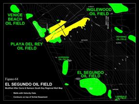 Playa Vista Example
Viewable Report - (April 2000) - /Report-04-2000/index.html
Viewable Report - (Regional) - /Regional/index.html
Of the examples cited above, the Playa Vista project conducted in Los Angeles, California is one of the most extensive and complete soil gas investigations ever conducted, and provides excellent material for illustrating the importance of higher density sampling(Jones et al., 2002). Examples from this investigation have adequate detail for defining the complexities that interconnect the vadose zone and groundwater gases with their associated deeper gas sources. The bubbling seep in Figure 1 was included to show just how small the exit point of a macro-seep can be, and this is quite typical. This macro-seep occurs in the Ballona Creek near the confluence of the Centinela and Ballona Creeks within the Playa Vista area of Los Angeles. The Playa Vista site, shown in yellow on Figure 64, is a 1087 acre development site that is currently being built on the old Howard Hughes airport site just north of Los Angeles International Airport, where the “Spruce Goose” was designed and constructed.
One of the main environmental problems with this site is that it contains numerous methane gas macro-seeps that lie within 2000 feet of the Playa del Rey Underground Gas Storage Field. Chemical and isotopic analysis of seepage gases taken from the bubbling seeps in Ballona Creek were initially collected and analyzed in 1993.
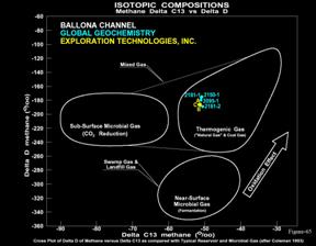 Seeps from this
same area were collected and analyzed seven years later in 2000 with excellent
repeatability (see Figure 65). The composition of these gases suggests a
mixture of biogenic and thermogenic gases.
Seeps from this
same area were collected and analyzed seven years later in 2000 with excellent
repeatability (see Figure 65). The composition of these gases suggests a
mixture of biogenic and thermogenic gases.
Monitor wells installed adjacent to Ballona Creek on the development site confirmed the presence of large methane concentrations in the groundwater aquifer at 50 feet below the surface and suggested that the methane charged area might be widespread. In response to the possibility that these gases could be leaking storage field gases, coupled with the potential for earthquakes, the Los Angeles Department of Building & Safety (LADBS) commissioned an extensive environmental assessment over the development site. This assessment included both regional and detailed soil gas surveys, the installation of forty-one 50-foot deep monitor wells and one hundred and twenty-two Geoprobe vent wells. The extensive seepage found by this assessment lead to a 3-D seismic survey, conducted to map potential fault conduits. An extensive report is available upon request from ETI.
Illustrations and excerpts from this investigation will paint a picture of the spatial variability exhibited by macro- and micro-seeps. This variability is basically controlled by a complex vadose zone/groundwater system that provides vertical migration pathways which control the distribution of the seeps. This complexity is significantly increased by the fact that the surficial sediments have a geologic history that is generally independent of the deeper geological systems that are the source of the seeping gases. Given this overall complexity, it is nevertheless observed that the seeps are generally vertical with respect to their deeper sources. This data set also demonstrates the effects of near-surface biological degradation that occur, not only in the saturated zone, but in the unsaturated (vadose) zone as well. The biological processes can complicate the relationship between methane and CO2, both of which can be generated independently. Methane also behaves more like an ideal gas within the vadose zone, where CO2 does not because it can be attenuated by groundwater due to its large solubility as compared to methane. This behavior results in CO2 having a more complex relationship than the hydrocarbon gases.
A four-foot deep soil gas survey conducted over a portion of the Playa Vista development site will be used to illustrate some of these very complex relationships. This soil gas data set shown in Figure 66 consists of 812 samples collected on 100-foot grid spacing. The purpose of the soil gas survey was to provide baseline data to determine the distribution and magnitude of methane soil gas anomalies in the near surface directly underlying the planned construction area. The collection procedure and analytical package was also designed to determine if there were any associated methane homologs (ethane, propane, or butanes) from a deep thermogenic source. Previous soil gas samples collected using a Geoprobe and analyzed by standard environmental laboratory procedures had been unable to detect these critical methane homologs. Resampling of the site using collection and analysis procedures developed for exploration found that these C2+ components were present in all of the methane soil gas anomalies, confirming that the gas seepage on this site contains some thermogenic gases from a mature subsurface source.
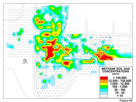 (Figure 66 - High Resolution Map from Original Report)
As shown on Figure 66, the concentration of methane in the soil gas is highly variable over the survey area. Values range from background (< 2 ppmv) to over 900,000 ppmv (90%). The highest contour interval drawn on the methane map is the upper explosive limit 150,000 ppmv (15%), and the next contour interval is 25% of the lower explosive limit or 12,500 ppmv (1.25%). These specific values were chosen for contouring the data in order to distinguish areas where the concentration is above these two levels of safety concern. However, it should be noted that these values are significantly below the highest values measured, which range from 25% to as much as 98% methane. This data also provides insight into the relationship between macro- and micro-seeps, and demonstrates how macro-seeps grade into micro-seeps. It is very important to note that this variation in magnitude occurs over a very small spatial distance. This is caused by the fact that the vertical gradient, driven by pressure, is almost always greater than the lateral gradient, where diffusion plays a larger role. This large difference in dynamic range means that non-linear contour intervals are usually required to properly represent soil gas magnitudes in a contour map format. Note that the lower contour values used to delineate the edges of the largest magnitude seeps are orders of magnitude less than those used to represent the larger magnitude seeps. The obvious inference is that fairly high density sampling is almost always required to find macro-seepage locations, where flux measurements can be made in the most effective and efficient manner.
Areas with anomalous methane concentrations (greater than 12,500 ppmv) are spread over a large portion of the survey area. In spite of their frequent occurrence, most contiguous anomalies consist of only one or two sites on 100 foot centers. There are, however, two anomalous areas that extend 900 - 1000 feet in length and 200 - 400 feet in width. In spite of the frequent occurrence of these large magnitude seeps with methane greater than 12,500 ppmv, their total area was found to cover only ~ 1.5% of the entire 1087 acre Playa Vista site. Smaller methane anomalies generally occur north of Jefferson Avenue, although, there are some macro-seeps in this area. Soil gas values over most of the remainder of the site are more typical of normal soil gas concentrations, (Jones et al. 2000).
Methane concentrations in the 25 - 90% range at a depth of only four feet generally cannot be sustained without active gas flow from depth. Methane is too volatile to be sustained at these levels without an active source. In this case, advective gas flow has been confirmed within the vicinity of many of the large magnitude seeps by means of visual observations of bubbles at the surface after flooding rains; in areas which are permanently water covered; and also in water saturated areas that overlap the largest soil gas seeps. The low-lying marshy environment of the surface on this site opens up the possibility that these gas seeps measured at a depth of only four feet could be biogenic gas generated in the marshy surface sediments. However, the chemical and isotopic composition of the bubbling gas seeps proves that at least part of this gas is more mature thermal gas from depth, and the presence of ethane in both the bubbling seeps and in the surface soil gases confirms this conclusion, since ethane is not generated via biogenic processes. However, none of these observations proves that the soil gases, the bubbling seep gases in the Ballona Creek, or the gases in the monitor wells have a common source.
The only way to determine the relationship of the soil gas seeps to the gases in the groundwater is to measure the content of methane and other gases present in the groundwater directly under these soil gas anomalies. For this purpose, a total of 41 monitor wells were installed. The primary groundwater aquifer (the Ballona aquifer) is a basal lithologic unit composed of sand and gravel that is generally referred to as the 50-foot gravel. This gravel aquifer is approximately 15 feet thick beneath the site and dips to the west toward the gas storage field. Previous interpretations regarding the gas in the aquifer had probably migrated updip from the storage field. The thickness, west dip and extremely high permeability of the 50-foot gravel aquifer suggested that this might be a reasonable possibility, provided that gas from the storage field was leaking into the aquifer in a downdip location relative to where these seeps have been found on the construction site.
An array of 41 monitor wells, screened in the 50-foot gravel aquifer, were installed during March 2000 in areas of high near-surface methane anomalies delineated by the soil gas survey. The first sign of significant levels of gas in the aquifer was demonstrated when several of the wells directly underneath the larger soil gas anomalies blew water 40 feet into the air when penetrated by the drill. Once the monitor wells were installed and completed, they were sampled using a sampling protocol that involved the collection of free gas bubbles in an inverted bottle and a dissolved gas sample collected from successive well volumes pumped from each well over a period of time. The average well volume is approximately 10 gallons of water. The water flow rate used was approximately ½ gallon per minute. This methodology allowed multiple free gas and dissolved gas samples to be collected over time from different well volumes. When possible, five or more well volumes from each well were removed and sampled.
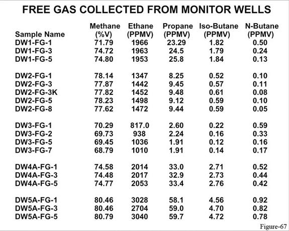 This sampling protocol then
provided representative water samples from the aquifer that were stable and
consistent with respect to one another, as shown on Figure 67. The free gas
and dissolved gas samples were collected into 125 ml glass bottles that were
then analyzed for both their chemical and isotopic compositions, including
their methane through hexane vapors and the permanent gases nitrogen, oxygen,
carbon dioxide, helium, argon, hydrogen and carbon monoxide. With this
procedure, independent and separate samples from successive well volumes could
be averaged to provide a measurement of the methane gas levels contained in the
groundwater adjacent to each monitor well. These average values were posted
and contoured to determine the actual distribution of the methane gas in the
50-foot gravel aquifer.
This sampling protocol then
provided representative water samples from the aquifer that were stable and
consistent with respect to one another, as shown on Figure 67. The free gas
and dissolved gas samples were collected into 125 ml glass bottles that were
then analyzed for both their chemical and isotopic compositions, including
their methane through hexane vapors and the permanent gases nitrogen, oxygen,
carbon dioxide, helium, argon, hydrogen and carbon monoxide. With this
procedure, independent and separate samples from successive well volumes could
be averaged to provide a measurement of the methane gas levels contained in the
groundwater adjacent to each monitor well. These average values were posted
and contoured to determine the actual distribution of the methane gas in the
50-foot gravel aquifer.
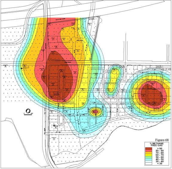 (Figure 68 - High Resolution Map from Original Report)
The average methane concentrations in the free gas samples from the 41 monitor wells are shown in Figure 68. As the soil gas would suggest, nearly all of the wells contained some measurable methane, with the highest concentration of methane ranging up to nearly one hundred percent (99.7%). In general, the highest free gas concentrations of methane observed in the wells is in excellent agreement with the soil gas. However, it is interesting to note that there is not a direct correlation that would indicate that Henry’s law is controlling the relationship between the free gases and the headspace (dissolved gases in the groundwater). A very good example is provided by MMW-211, which had enough free gas to blow the water to a height of over 40 feet into the air when the well was initially drilled. When finally sampled, this well had only about 60% methane in the free gas in the well and 17 mg/l of dissolved gas in the water sample. In contrast monitor well MMW-226, placed on the edge of the anomalous methane area where the soil gas methane was only 1300 ppm, had 99.7% methane in the free gas in the aquifer and 48.3 mg/l (saturation) of dissolved gas in the water sample. Thus one of the largest soil gas anomalies (89.2% methane) occurred where monitor well 211 was placed, yet methane in the groundwater under this site was not saturated. The fact that the aquifer is not saturated with gas at this location suggests that an independent gas pocket that is not in equilibrium with the groundwater was the likely cause of the blowout in monitor well 211, and that independent gas migration pathways must be channeling through the groundwater.
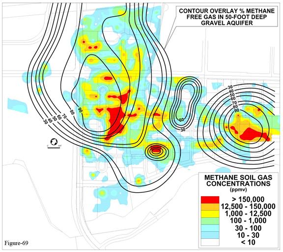 Figure 69 provides an overlay of
the methane groundwater contours on top of the soil gas methane anomalies.
There is obviously a very strong spatial correlation between the soil gas
anomalies and the groundwater anomalies, in spite of the fact that there is gas
migration in the vadose zone above the aquifer that is independent of the gases
contained within the aquifer. There is an obvious relationship between the two
independent data sets, yet the groundwater is clearly not the sole source of
the four foot deep soil gases. This obvious correlation requires that they
have a deeper and common source that must lie below the groundwater aquifer.
This relationship proves that the dominant migration of gas is vertical, but
that different localized parameters are controlling the individual aquifer and
soil gas concentrations. This correlation between the methane gas
concentrations in the groundwater and the soil gases also suggests that there
is very little lateral gas migration within the aquifer, reducing the likelihood
that the gas storage field is a source for these gases. This fits very well
with our previous experience in exploration surveys that had always suggested
that groundwater flow almost never has any controlling effect on the
distribution of gases within the near surface strata. The time for gas to pass
vertically through an aquifer is very short when compared to the time for
groundwater to move laterally.
Figure 69 provides an overlay of
the methane groundwater contours on top of the soil gas methane anomalies.
There is obviously a very strong spatial correlation between the soil gas
anomalies and the groundwater anomalies, in spite of the fact that there is gas
migration in the vadose zone above the aquifer that is independent of the gases
contained within the aquifer. There is an obvious relationship between the two
independent data sets, yet the groundwater is clearly not the sole source of
the four foot deep soil gases. This obvious correlation requires that they
have a deeper and common source that must lie below the groundwater aquifer.
This relationship proves that the dominant migration of gas is vertical, but
that different localized parameters are controlling the individual aquifer and
soil gas concentrations. This correlation between the methane gas
concentrations in the groundwater and the soil gases also suggests that there
is very little lateral gas migration within the aquifer, reducing the likelihood
that the gas storage field is a source for these gases. This fits very well
with our previous experience in exploration surveys that had always suggested
that groundwater flow almost never has any controlling effect on the
distribution of gases within the near surface strata. The time for gas to pass
vertically through an aquifer is very short when compared to the time for
groundwater to move laterally.
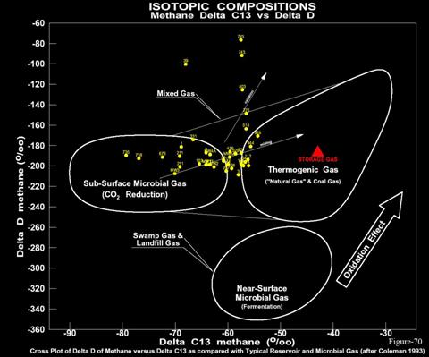 A plot of the carbon and hydrogen
isotopic compositions of the methane samples from the groundwater monitor wells
shown in Figure 70 indicates that most of the samples fall within the mixed
zone between the subsurface microbial gas and the thermogenic gas zone. This
suggests that these samples represent different mixtures of thermogenic gas and
biogenic methane. A simple way to determine which samples contain the most
thermogenic gas can be demonstrated by cross plotting the propane/methane ratio
(propane is never generated biologically) against the carbon 13/12 isotopic
ratio, as shown by Figure 71a.
A plot of the carbon and hydrogen
isotopic compositions of the methane samples from the groundwater monitor wells
shown in Figure 70 indicates that most of the samples fall within the mixed
zone between the subsurface microbial gas and the thermogenic gas zone. This
suggests that these samples represent different mixtures of thermogenic gas and
biogenic methane. A simple way to determine which samples contain the most
thermogenic gas can be demonstrated by cross plotting the propane/methane ratio
(propane is never generated biologically) against the carbon 13/12 isotopic
ratio, as shown by Figure 71a.
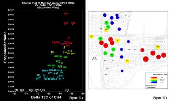 On this dot map plot on Figure
71b the methane concentrations have been made proportional to the size of the
dots on the map view and the colors provide the relative amounts of biogenic
(blue) versus thermogenic (red) gas. These two plots indicate that the larger
concentrations of methane in the groundwater contain the most thermogenic gases
from depth. The map view even shows that the gases containing the largest
mixtures of biogenic gas occur on the edges of the thermal gas anomalies. Thus
the biogenic gases might have been
generated within the 50 foot gravel aquifer, caused by the
reduction of oxygen in the groundwater related to the presence of the thermogenic gas seeps. In any case the presence of independent thermogenic seeps suggests that the thermogenic gases
must be migrating up into the aquifer from deeper formations.
On this dot map plot on Figure
71b the methane concentrations have been made proportional to the size of the
dots on the map view and the colors provide the relative amounts of biogenic
(blue) versus thermogenic (red) gas. These two plots indicate that the larger
concentrations of methane in the groundwater contain the most thermogenic gases
from depth. The map view even shows that the gases containing the largest
mixtures of biogenic gas occur on the edges of the thermal gas anomalies. Thus
the biogenic gases might have been
generated within the 50 foot gravel aquifer, caused by the
reduction of oxygen in the groundwater related to the presence of the thermogenic gas seeps. In any case the presence of independent thermogenic seeps suggests that the thermogenic gases
must be migrating up into the aquifer from deeper formations.
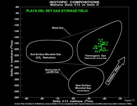 The soil gas and groundwater
methane maps show no obvious migration links to the nearby gas storage field.
As a final, even more definitive evaluation, nine of the gas storage and
observation wells were sampled and analyzed for their chemical and isotopic
compositions which are plotted on Figure 72. A direct comparison of this
chemical and isotopic data with the surface soil gases and with the gas data
from the Ballona gravel aquifer monitor wells clearly demonstrates that the gas
storage wells are isotopically and chemically different from the Playa Vista
gases. Thus the overwhelming evidence demonstrates that the gas storage field is
not the source of the gases.
The soil gas and groundwater
methane maps show no obvious migration links to the nearby gas storage field.
As a final, even more definitive evaluation, nine of the gas storage and
observation wells were sampled and analyzed for their chemical and isotopic
compositions which are plotted on Figure 72. A direct comparison of this
chemical and isotopic data with the surface soil gases and with the gas data
from the Ballona gravel aquifer monitor wells clearly demonstrates that the gas
storage wells are isotopically and chemically different from the Playa Vista
gases. Thus the overwhelming evidence demonstrates that the gas storage field is
not the source of the gases.
The most obvious alternative source for thermogenic gases under this site would then be sources such as the shallow natural gas sands within the Upper Pliocene Pico Formation. Shows encountered in the non-commercial wells drilled near the site occurred from numerous sands found as shallow as 510 feet to as deep as 3434 feet. An evaluation of reports from these abandoned wells revealed that the Universal City Syndicate, Inc. Vidor #1, located on the western edge of the area, was drilled to a total depth of 5960 feet and was plugged and abandoned as a dry hole in 1931. Shallow natural gas was encountered while drilling at depths of 1140 to 1150 feet. The well blew out on August 27, 1930, at an estimated rate of 5000 MCF of gas per day, while drilling at 1821 feet. On May 2, 1931 the well blew out a second time while drilling at a depth of 5960 feet. As shown on Figure 69, there was a small soil gas anomaly found near the abandoned well casing, and there was some methane gas in the 50-foot gravel aquifer in monitor well MMW-514 which was placed to evaluate this area. However, neither the soil gases nor the groundwater wells suggest that this plugged and abandoned well is a conduit that could be responsible for this extensive complex of gas seeps. If this well were a conduit, then the gases leaking up along the abandoned casing should exhibit a lateral migration pathway within the gravel aquifer. The strong spatial correlations between the soil gases and the gases concentrated in the various monitor wells argue against this possibility. An evaluation of many of the deep production wells from the area indicated that the observations made in the Universal City Syndicate, Inc. Vidor #1 were common throughout the general area, and gases observed in formations encountered by these wells at depths of 1000 to 6000 feet appear to provide the most likely source for the surface gas seepage at Playa Vista.
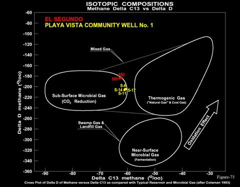 Additional investigations
indicated that natural gas had been discovered between depths of 1,500 ft to
4,700 ft, in the Pico and Repetto sands of the El Segundo field, which is on a
similar structural trend only 4.5 miles southwest of Playa Vista. The analyses
of two Pico gas samples from this field showed that they are very similar to
the gases at Playa Vista. This field has produced about 23 billion cubic feet
of gas, and provides an indication of the possible magnitude of the gas
accumulations that could exist beneath Playa Vista. During the final
re-abandonment of the Universal City Syndicate, Inc. Vidor #1 well, gas samples
were obtained from the Silverado fresh drinking water aquifer located at a
depth of 668 to 760 feet. As shown on Figure 73, the isotopic composition of
the El Segundo gases are in good agreement with those of gases in the 50 foot
gravel aquifer and with those of the gases obtained from the Silverado,
suggesting that these deeper formation gases are the most likely source for the
shallow gas seepage observed at Playa Vista.
Additional investigations
indicated that natural gas had been discovered between depths of 1,500 ft to
4,700 ft, in the Pico and Repetto sands of the El Segundo field, which is on a
similar structural trend only 4.5 miles southwest of Playa Vista. The analyses
of two Pico gas samples from this field showed that they are very similar to
the gases at Playa Vista. This field has produced about 23 billion cubic feet
of gas, and provides an indication of the possible magnitude of the gas
accumulations that could exist beneath Playa Vista. During the final
re-abandonment of the Universal City Syndicate, Inc. Vidor #1 well, gas samples
were obtained from the Silverado fresh drinking water aquifer located at a
depth of 668 to 760 feet. As shown on Figure 73, the isotopic composition of
the El Segundo gases are in good agreement with those of gases in the 50 foot
gravel aquifer and with those of the gases obtained from the Silverado,
suggesting that these deeper formation gases are the most likely source for the
shallow gas seepage observed at Playa Vista.
An independent assessment was also made of the geological and geophysical characteristics of the formations at Playa Vista in an effort to understand the nature of the structure and stratigraphy of the subsurface gas sources and the gas migration pathways. A high-resolution 2D seismic line, located along Jefferson Boulevard provides an image of the shallow subsurface down to a depth of about 2,000 ft. A 3D seismic survey was also carried out to image the deeper section, extending to about 8,000 ft. Figure 74 shows a contour map of the soil gas anomalies plotted directly over the 2-D seismic section. Note the seismic wipe-out zones (lack of reflectors) in the sections that directly underlie the two larger anomalies. This is a typical response that is often associated with subsurface oil and gas reservoirs. It is caused by attenuation of the seismic waves related to the presence of gas filled fractures. This seismic response provides further support of a deep source origin of the surface seepage and water well gases.
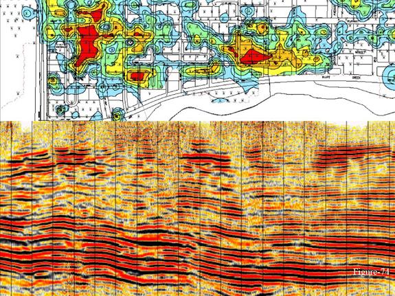
Vadose Zone Vertical Migration Pathways and Interferences
An extensive program of drilling and testing of vent wells and monitor wells was carried out within the upper 50 feet of sedimentary cover underlying these gas-charged areas in an effort to characterize the nature and source of these thermogenic gases within the vadose zone/groundwater system. Hydrologic measurements in the 50-foot gravel aquifer indicated that it is a confined aquifer, allowing the possibility that the finer grained sediments capping the 50-foot gravels might provide a seal, allowing free gas pockets to accumulate just below this interface. The presence of such gas pockets could explain the lack of a direct magnitude relationship between the gases dissolved in the 50-foot gravel aquifer and the surface seeps. If these shallow pockets could be found and drained, then the surface gas venting could be significantly reduced, or perhaps even eliminated. In this case, gas venting wells could be permanently installed and monitored to mitigate the gas and insure a safe environment.
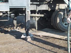 The first test
performed at soil gas site 207 was very successful. A CPT borehole was pushed
to 66 feet below surface at this site. When the probe rods were pulled up to
60 feet subsurface, the well discharged about one gallon of water and then
flowed free gas at the rate of 10 liter/minute for 69 hours, until destroyed in
an unsuccessful attempt to replace the CPT probe rods with a monitor well.
Similar results were found on the second attempt at soil gas site 211. The positive
gas pressure is shown on Figure 75. Over 173 CPT boreholes were pushed to
refusal at the top of the Ballona Gravel using a CPT (Cone Penetrometer)
method. Once the top of the gravel was determined by the point of refusal, the
drive rods could be opened to measure pressure and vent any free gas. Whenever
free gas pockets were encountered, the drive rods were left in place and the
gas was allowed to vent. Unfortunately most of these attempts to install gas
vent wells failed because the silts at the top of the 50-foot gravels were too
unconsolidated to remain open. The wells were clogged by unconsolidated
clastic sediment and invaded by water, which then shut off the gas flow. Many
unsuccessful attempts were made to solve this mechanical production problem.
Unfortunately, gas production was too sporadic and unpredictable to be
effective.
The first test
performed at soil gas site 207 was very successful. A CPT borehole was pushed
to 66 feet below surface at this site. When the probe rods were pulled up to
60 feet subsurface, the well discharged about one gallon of water and then
flowed free gas at the rate of 10 liter/minute for 69 hours, until destroyed in
an unsuccessful attempt to replace the CPT probe rods with a monitor well.
Similar results were found on the second attempt at soil gas site 211. The positive
gas pressure is shown on Figure 75. Over 173 CPT boreholes were pushed to
refusal at the top of the Ballona Gravel using a CPT (Cone Penetrometer)
method. Once the top of the gravel was determined by the point of refusal, the
drive rods could be opened to measure pressure and vent any free gas. Whenever
free gas pockets were encountered, the drive rods were left in place and the
gas was allowed to vent. Unfortunately most of these attempts to install gas
vent wells failed because the silts at the top of the 50-foot gravels were too
unconsolidated to remain open. The wells were clogged by unconsolidated
clastic sediment and invaded by water, which then shut off the gas flow. Many
unsuccessful attempts were made to solve this mechanical production problem.
Unfortunately, gas production was too sporadic and unpredictable to be
effective.
Free gas was generally present somewhere in the upper 50 feet of sediments within the areas having the largest methane soil gases. This free gas was, however, not easily found, nor vented from these unconsolidated sediments. Gas could not even be successfully vented from the vicinity of many of the largest macro-seep areas. Initially the vent wells were installed on a 100 foot spacing, as was also used for the soil gas survey, but as failures began to occur, this spacing was reduced to as close as 10 foot centers. A classic example of this failure was demonstrated when three CPT wells were placed within 10 feet of a very large macro-seep, and none were capable of venting gas from the gravel aquifer. Even more impressive was the fact that this macro-seep had been missed by the 100 foot centered soil gas survey, and only discovered after a heavy rain had flooded the surface, allowing visual observation of the bubbles.
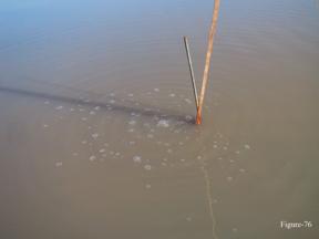 On Figure 76 is
shown an example of seeps that had not been found until the surface was
flooded. Soil gas sampling on 100 foot centers had missed this seep.
On Figure 76 is
shown an example of seeps that had not been found until the surface was
flooded. Soil gas sampling on 100 foot centers had missed this seep.
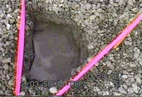 A flux
measurement revealed that this macro-seep was venting 9 liter/minute of free
gas. Since this vent was not visible when the surface was not flooded, a
semi-permanent flux measuring station was installed (see Figure 77) at this
location by digging a 24-inch 10-foot deep hole, which was cased with 24-inch
PVC pipe and filled with gravel.
A flux
measurement revealed that this macro-seep was venting 9 liter/minute of free
gas. Since this vent was not visible when the surface was not flooded, a
semi-permanent flux measuring station was installed (see Figure 77) at this
location by digging a 24-inch 10-foot deep hole, which was cased with 24-inch
PVC pipe and filled with gravel.
Two gas samples from this well were analyzed for their chemical and isotopic compositions and found to contain 97.68% and 97.66% methane. The carbon dioxide levels were 0.72% and 0.67%, respectively, providing nearly 99% of the total gas when added to the methane. Ethane and propane were also present in the normal range at 0.34% and 0.0046% (3400 and 46 ppmv). Carbon isotopes of the contained ethane were –20.08 and –20.01 parts per thousand with respect to the PDB standard. Comparison with the 50-foot Ballona gravel monitor wells indicates that these gases are nearly identical to those contained within the aquifer at depth. They contain almost no air and show no sign of biodegradation. Clearly these samples are vertically discharging directly from the Ballona gravel aquifer without any additional degradation related to residence within the upper 50 feet of sediments. As noted above, three CPT wells placed only 10 feet away from the bubbling well found no gas pockets in the gravel, indicating that in this case, the gravel is merely a transmission zone. The source of this gas must lie below the gravel.
Numerous other observations similar to the above example demonstrated the very high spatial variability of these gas vents. In an attempt to improve the placement of vent and monitor wells, additional infill soil gas samples were collected within the main seepage areas. As with exploration surveys, decreasing the sampling interval always reduces the areal size of the contoured anomalies. A closer-spaced sampling grid can also result in the discovery of more individual (smaller sized) anomalies. This is a very important point because soil gas anomalies don’t have to occupy a large areal extent in order to provide a significant gas source under a building.
Flux Pipes and Footprints
The best method for measuring the actual flux into the atmosphere would be to construct a large flux chamber that would cover the entire area of interest. This, of course is not practical. In fact, soil gas surveys take advantage of the fact that the earth actually serves as a large flux chamber. When advective flow exists (driven by pressure), gas migrates toward the surface, enters the vadose zone and fills the permeable pathways with gas. A breakthrough into the atmosphere provides pressure relief that acts to reduce lateral flow. Finding these breakthrough points is nearly impossible using standard flux chambers because of the very small size of both the seeps and the chambers. The soil gas survey, on the other hand, offers a practical approach for finding these natural flux locations or “flux pipes”.
At the surface there is a natural equilibrium formed in which the gas flux from depth and the gas flux into the atmosphere must balance. The point or area at which the gas flux into the atmosphere is maximized is called the “flux pipe”. Lateral migration, both by advection and diffusion, will always occur around the “flux pipe”. This results in a soil gas anomaly with a stable “flux footprint”. While the “flux pipe” may be of a limited size and be difficult to find, the “flux footprint” has a larger areal extent which may be more easily located by the process of a soil gas survey. Flux footprints have concentrations which can be measured and contoured to provide direction toward the largest soil gas concentrations where the “flux pipe” is located.
During the course of the Playa Vista investigation numerous flux measurements were attempted using standard flux chambers. Forty such measurements (with very poor results) were carried out within the area discussed above where macro-seeps were later observed following a rain large enough to flood the surface. Over 140 bubbling macro-seeps were staked in this area, yet all had been missed by the flux chambers. This clearly demonstrated that the application of a limited number of measurements of any kind without any guidance from a soil gas survey is likely to fail. Data from such a survey could be misconstrued if used as evidence that macro-seeps are not present.
The initial, more regional soil gas survey shown in Figure 69 was conducted using 100 foot centers, which worked adequately for locating several flux footprints of potential macro-seepage. This spacing is, however, completely inadequate for placement of flux chambers. The reduction to 50 foot centers, with occasional infill provided a much better, but still incomplete estimate of the actual size and shape of the individual soil gas anomalies, or “flux footprints” within the areas that had been surveyed. The success of higher density sampling for locating additional macro-seeps, or “flux pipes” is demonstrated by the following examples where a more detailed grid of 50 feet, coupled with additional infill samples suggested by the soil gas results have established the presence of two new active gas flux areas or flux pipes.
Both of these examples are within areas where the groundwater data had indicated that the 50-foot gravel aquifer was charged with gas, but where no large macro-seeps had been found by the 100-foot spaced soil gas survey. As these examples will show, large magnitude macro-seeps do exist within this area, but with much smaller “flux footprints”. Integration with the seismic data showed that some clay channels had been deposited in this area, reducing the number of migration pathways available.
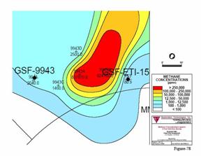 An expanded
detail, contour map for methane is shown in Figure 78, where methane
concentrations of 80.8 and 82.4% were found approximately 10 feet apart at
Sites 9943A and 9943B. In contrast, the largest values surrounding these two large
macro-seep sites have methane concentrations, which are generally less than
2000 ppmv (0.2%), and just 10 feet to the east is site 153, where only 80.9
ppmv (0.0081%) was measured. When establishing the more detailed grid, site
9943 was placed halfway between sites 153 (80.9 ppmv) and 154 (612.5 ppmv).
The value of 2040 ppmv measured at site 9943 was larger than either of the two
original sites, but clearly did not find a macro-seep in this area; however,
previous observations had noted free gas bubbling to the surface in this
general area. The extra infill sample (9943A) added halfway between sites 9943
and site 153 found a concentration of 807,870 ppmv, confirming the existence of
a large magnitude soil gas anomaly, or “flux footprint” in this area. A second
offset sample at site 9943B provided additional confirmation, and indicated
that the soil gas anomaly associated with this macro-seep occupies an area at
least 10 feet in width. Sites 9943C and 9943D were added to further define the
northern and western edges. When these infill sites were placed into the
regional map it was evident that additional samples should have been placed to
the northeast, toward sites 9952C and 9940. A potential northeast – southwest
alignment is suggested by this soil gas data. Precise definition of flux pipes
such as these could be expedited by the use of a mobile laboratory to let the
data drive the sampling on a much more real time basis.
An expanded
detail, contour map for methane is shown in Figure 78, where methane
concentrations of 80.8 and 82.4% were found approximately 10 feet apart at
Sites 9943A and 9943B. In contrast, the largest values surrounding these two large
macro-seep sites have methane concentrations, which are generally less than
2000 ppmv (0.2%), and just 10 feet to the east is site 153, where only 80.9
ppmv (0.0081%) was measured. When establishing the more detailed grid, site
9943 was placed halfway between sites 153 (80.9 ppmv) and 154 (612.5 ppmv).
The value of 2040 ppmv measured at site 9943 was larger than either of the two
original sites, but clearly did not find a macro-seep in this area; however,
previous observations had noted free gas bubbling to the surface in this
general area. The extra infill sample (9943A) added halfway between sites 9943
and site 153 found a concentration of 807,870 ppmv, confirming the existence of
a large magnitude soil gas anomaly, or “flux footprint” in this area. A second
offset sample at site 9943B provided additional confirmation, and indicated
that the soil gas anomaly associated with this macro-seep occupies an area at
least 10 feet in width. Sites 9943C and 9943D were added to further define the
northern and western edges. When these infill sites were placed into the
regional map it was evident that additional samples should have been placed to
the northeast, toward sites 9952C and 9940. A potential northeast – southwest
alignment is suggested by this soil gas data. Precise definition of flux pipes
such as these could be expedited by the use of a mobile laboratory to let the
data drive the sampling on a much more real time basis.
The presence of two large magnitude soil gas anomalies located only 10 feet apart, when taken in context with the other anomalous samples indicates a very high potential for significant seepage under this area. It is important to note that these sites would probably never have been collected close enough for this confirmation without the visual observation of bubbles that had been noted earlier. Of even more significance, however, is the fact that this “flux footprint” demonstrates the presence of adequate conditions for vertical migration directly from the underlying gravel aquifer, and confirming the existence of a large macro-seep within an area that the regional soil gas survey missed.
Another excellent example of a very well-defined macro-seep was found by adding a grid of samples near monitor well MMW-04. This monitor well blew out for over an hour when it first penetrated the gravel aquifer. It also contained very anomalous free and dissolved gas concentrations in the water samples initially collected (ETI April 17, 2000 report). This well lies near the center of the > 90% methane contour on the groundwater map (Figure 71) and would appear to be a possible area where deep gas might be entering the gravel aquifer from below. It was puzzling then that the initial soil gas contour maps on 100 foot centers did not show a large soil gas anomaly vertically over this very anomalous area of the gravel aquifer, as the data from the aquifer would suggest. Only site 201 had noted the possible presence of an anomaly in this general area. In order to evaluate the potential for this gravel aquifer anomaly to be a gas source, an infill grid was placed between site 201 and monitor well MMW-04. Initially sites 004A through 004I were collected within the boundaries defined by sites 180, 181, 200 and 201, and only sites 004C and 004F showed appreciable values of 75.7% and 98.6% methane. Based on these initial infill results additional sites were added (up to 004Z).
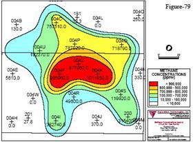
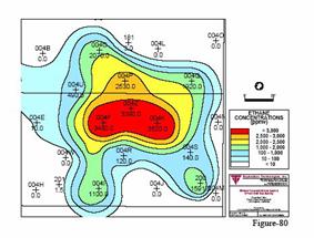
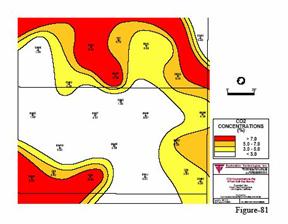
In order to properly display this anomaly, an expanded view of this infill grid using a scale of 20 feet to the inch has been included in Figures 79, 80 and 81 for the methane, ethane and carbon dioxide. This infill grid confirms one of the most significant and well defined anomalies mapped by these soil gas surveys, with methane concentrations of 75.8%, 97.8% and 100%. These are three of the largest soil gas concentrations measured anywhere on the site. Ethane concentrations are also very large and were equivalent to those found in the 50-foot gravel aquifer.
Although carbon dioxide has not been included or discussed in the previous examples, it was measured at all sites. This macro-seep shows the classic “halo” pattern that CO2 exhibits within a hydrocarbon macro-seep. Within the heart of the macro-seep the CO2 is reduced for two reasons. One is that the oxidation of the organic food source (i.e. methane in this case) has depleted the oxygen faster than it can diffuse in from the atmosphere, The second factor that acts to reduce the oxygen concentration, and thus the CO2 generated is that in an advective seep the oxygen can also be displaced and diluted by the seepage gases. As shown by this example, the maximum soil gas CO2 concentrations occur near the edge of the macro-seep where the mix of available oxygen and fuel (methane) is adequate for microbial activity. Within a very short distance from the edge of the macro-seep the CO2 drops to typical background values of 0.5 to perhaps 2 or 3%. These degradation processes control the quantity of CO2 in the soil gas, and can cause interference in any monitoring program designed to measure CO2 that has migrated from depth. These CO2 halo patterns can only be recognized and properly defined using fairly high density soil gas surveys, generally on the order of 10’s of feet. On wider spacing, even as close as 100 feet, they are often not recognized. Since these biodegradation-related CO2 concentrations can range upwards of 15 to 30%, they are very significant, and must be properly documented within any carbon sequestration monitoring program. While it is true that most carbon sequestration monitoring programs may not be associated with such macro hydrocarbon flux, there will exist abundant organic material from numerous sources over most old oil fields that can be a source of biogenic CO2. All surface sources of CO2 should be evaluated prior to CO2 injection.
Once this anomaly was defined by the infill soil gas survey, further examination of the ground at this site did result in the location of several macro-seeps of small areal extent located between the larger magnitude samples.
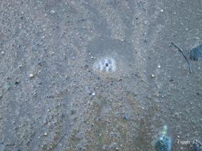 As shown in Figure
82, small macro-seeps like this one were photographed and viewed over several
days when conditions were wet enough to allow favorable visual observation.
As shown in Figure
82, small macro-seeps like this one were photographed and viewed over several
days when conditions were wet enough to allow favorable visual observation.
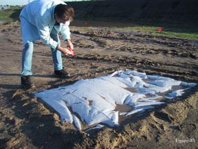 For further
testing, a small 4 foot by 4 foot plastic tent was placed over this site and
sealed on its edges by burial in the soil (see Figure 83). Although soil
conditions appeared to be too damp and tight to allow free gas bubbles to easily
appear at the surface at this site, the soil gas data proved that there was a
soil gas concentration of 98.6% methane at four feet below surface. Ambient
air samples were taken under the tent over the next two days in order to
establish whether or not there was any positive flux at this site. Within 24
hours the tent had ballooned up, and a concentration of 4.73% methane had
developed under the tent. Thus, even though the venting was not easily visible,
these observations indicated that seepage was occurring and would have been
overlooked without a more aggressive sampling program.
For further
testing, a small 4 foot by 4 foot plastic tent was placed over this site and
sealed on its edges by burial in the soil (see Figure 83). Although soil
conditions appeared to be too damp and tight to allow free gas bubbles to easily
appear at the surface at this site, the soil gas data proved that there was a
soil gas concentration of 98.6% methane at four feet below surface. Ambient
air samples were taken under the tent over the next two days in order to
establish whether or not there was any positive flux at this site. Within 24
hours the tent had ballooned up, and a concentration of 4.73% methane had
developed under the tent. Thus, even though the venting was not easily visible,
these observations indicated that seepage was occurring and would have been
overlooked without a more aggressive sampling program.
Subsequent testing for gas that could be vented from the underlying gravel aquifer was unsuccessful at this site. Five CPT gas vent boreholes were attempted near this location, three found no gas (TVW-35, TVW-75 and TVW-94), and two found only a small amount. TVW-93 was tested from the top of the gravel at 54.5 feet bgs to the surface and found a minor gas pocket at 24.2 feet. TVW-104 never found a point of refusal and was pushed to 82 feet bgs, although traces of gas were recorded as present from 62 to 82 feet. Clearly there is no gas pocket in the 50-foot deep gravel aquifer at this location, yet gas is venting at the surface. Five test wells, sampled from the gravel to the surface for free gas pockets within this soil gas anomaly strongly suggests that deeper gas is venting directly through the Ballona gravels, and through the upper 50 feet of sedimentary cover at this location without significant accumulation in intermediate reservoirs.
These two examples demonstrate that, while the presence of free gas bubbles helps in finding macro-seeps, there could be no assurance that this method would be sufficient for insuring that all of the macro-seep areas had been found and mapped. Thus while mapping the presence of bubbles is conclusive evidence of advective flow, a lack of bubbles cannot be used to assume that advective flow is not occurring. Previous discussion focused on the fact that the very largest soil gas anomalies did not directly overlay the largest groundwater contours shown in Figure 69. Initial suggestions included lateral migration of the soil gases from the gravel aquifer, in spite of the fact that soil gases migrate vertically. Subsequent groundwater potentiometric measurements show that the groundwater was flowing north into the Ballona Channel. This is also obvious from the groundwater contours. Although macro-seeps were not initially found directly over this large groundwater methane anomaly and suggested that this area did not contain advective seeps, higher density surveys revealed that they were indeed present.
The following example from a portion of the Playa Vista survey, as shown in Figures 84a and 84b, further demonstrates the importance of sample spacing for the purpose of precisely defining the locations of macro-seepage locations. It is at these locations that carbon sequestration flux monitoring stations should be located if they are to define the magnitude of leakage from a subsurface reservoir. A small portion of the initial Playa Vista soil gas data, taken from Figure 66, is reproduced on the left in Figure 84a. The distance between the sample points in Figure 84a is 100 feet and the contour intervals are 150,000, 12,500, 1000, 100, 30 and 10 ppm. A more detailed grid, shown in Figure 84b includes the results of integrating the large seeps shown in Figure 79 into the regional 100-foot data. Although this contour map looks very different from the lower density map, it covers the same areas as the map in Figure 84a. The change in the grid on the right is the result of collecting additional samples on approximately 50 to 25 foot spacings as needed to better define the initial anomalies encountered on the 100 foot grid. This large group of anomalous samples shown on Figure 84b in red appears to cover a larger footprint that most of the other macro-seeps encountered, , This group of “flux pipes” lies approximately 25 to 50 feet east of monitor well MMW4 that had blown out when first drilled to the top of the 50 foot gravel. It’s not known whether this cluster of soil gas macro-seeps marks the vertical location where the gas enters the bottom of the 50 foot gravel, but that appears likely. Monitor well MMW4 was located just close enough to encounter the gas bubble that developed within the gravel adjacent to the vertical migration pathway associated with this macro-seep. Once this well had vented, it did not recharge with free gas even though it is within 25 feet of a “flux pipe”.
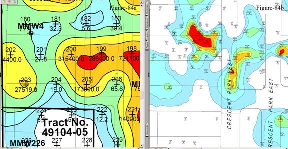 (Figure 84a - High Resolution Map from Original Report)
(Figure 84b - High Resolution Map from Original Report)
The most important point to be made from this example is the very significant difference in the location and shape of the anomalies defined by these two contour maps. As stated earlier with regard to exploration survey examples, grids with increased detail almost always reduce the areal extent of the anomalies. The large magnitudes found at soil gas sites 200, 199 and 198 were contoured as one large anomaly in Figure 84a. These were not insignificant seeps, ranging in concentration from 315,400, 286,600 and 721,100 ppm, respectively. However, by adding samples on a 50 foot spacing, even larger magnitude samples as well as many more background samples were encountered, splitting the “flux footprint” contoured on 100 foot spacing into three separate, larger magnitude, but much more localized “flux footprints” as shown by Figure 84b. The contour intervals in Figure 84b were changed to 250,000, 100,000, 50,000, 12,500, 1000 and 100 ppm in order to better illustrate the shapes of these three macro-seeps. Although changing the contour intervals did affect the shape of these three anomalies, the most important point to make is that the increased density made a critical difference as regards selecting locations where flux monitoring stations should be placed. Gas seepage is predominantly vertical because it is driven by pressure (which changes vertically, but not laterally). Flux measurements must be made within the well defined “flux footprint” of the seep in order to generate useful data.
If we have demonstrated anything in this document, it is that the strata overlying a petroleum reservoir are not isotropic, at least with regard to the paths of migrating gases from depth to the surface. On the contrary, such migration paths are localized and are defined by the geology and hydrogeology of the region. We also believe that their locations have been fixed by the seepage of thermogenic hydrocarbons over geologic time and that these are the pathways that carbon dioxide will travel when it leaks from its sequestration reservoir. This means that an arbitrarily placed sample location, be it for soil gas or flux measurement is unlikely to find meaningful results. Meaningful results can only be realized by defining the flux footprints and pipes with gridded soil gas surveys with additional detail added based on initial observations and other site specific conditions.
A review of the limited monitoring conducted to date over reservoirs studied for carbon sequestration (Nance et. al., 2005, Klusman, 2003, 2005) has revealed that the monitoring stations have been chosen without the use of gridded soil gas surveys to identify flux footprints and pipes in which meaningful measurements can be made. Identification of such locations at the surface over a sequestration reservoir can only be made from a representative data set (Popek and Kassakhian, 1998) of the soil gas concentrations over the entire area. Certainly over any candidate subsurface reservoir this will require gridded measurements with infill sampling as needed to precisely define the vertical migration pathways.
As pointed out in the introduction in this paper, petroleum reservoirs contain specific compounds, such as the ethane, propane and butane components which are uniquely characteristic of petroleum reservoir and source rock fluids. Experience has shown that these gases provide excellent tracers, so that, adding tracers is probably unnecessary, particularly when injecting CO2 into old oil or gas reservoirs. Thus, hydrocarbon reservoirs contain their own tracers, in the form of ethane through butanes, which are present in all petroleum reservoirs. Tracers could be employed much later in the process when leakages have been established and there is a need to determine residence and migration transit times. As shown in previous examples, helium has been used as a tracer for measuring the residence time of oxygen in an underground coal gas retort and the migration time for propane from an underground propane storage reservoir to transit to the surface.
A 100-foot sampling grid would obviously be considered a very detailed survey by the designers of current carbon sequestration monitoring programs. As demonstrated by the Playa Vista example, even this spacing may not be adequate for defining all of the “flux footprints” within this survey area. In contrast, only four monitoring sites were installed over the Frio injection site in Texas (Nance, et. al., 2005) and only 40 monitoring sites were placed on one mile centers over the TeaPot Dome Field in Wyoming (Klusman, 2005). The likelihood that any of these monitoring stations would intersect a vertical migration pathway is very small, and even if leakage exists, it would likely be missed by these few monitoring stations.
As noted earlier, numerous surface flux tests were conducted at Playa Vista using a standard flux chamber over portions of the area where the larger methane anomalies are located. The calculated flux values range from 0.000182 to 2.367 cubic feet of gas per square foot per day. As expected, the higher flux values correlate regionally with the underlying soil gas data. The larger values of ~2 cubic feet/square foot/day occur over visible macro-seeps where the largest and most extensive soil gas anomalies occur. Only background flux values were found over areas where the soil gas is uniformly low. However, because the flux chamber covers such a restricted surface area (approximately 1.75 ft2), it is possible for a single flux chamber measurement to fail at finding an advective seep, where the surface exit point may be very restricted in size and is not physically observable. As noted earlier, this did occur on the initial placement of the flux chambers when too few chambers were placed at random, and were not placed directly over macro-seeps located by soil gas surveys.
In contrast to flux chambers, soil gas surveys have the capability to approximately locate large magnitude soil gas anomalies and potentially macro-seeps without actually sampling the largest magnitudes in the area. A flux chamber, on the other hand, must be precisely placed in order to make an accurate flux measurement associated with an advective seep. These examples demonstrate the ability of soil gas sampling to approximately locate areas which must be searched for active vents before accurate flux measurements should be attempted. The flux chamber was designed to measure diffusive flux and does not accurately measure, nor easily locate advective flux sites. In order to achieve useable flux results without having a very large number of individual flux stations, it is imperative that the flux chamber measurements be guided by a soil gas survey to best define the locations for the flux measurements to be made.
Effects of Biodegradation and Moisture on Seepage Patterns
Early observations at Playa Vista made in some of the macro-seepage areas under dry conditions (when the surface was not flooded) illustrated some of the biodegradation effects that occur near the surface within the vadose zone. It appears that these biodegradation effects are likely caused by ambient air influx and/or soil moisture on the concentrations and compositions of these macro-seeps.
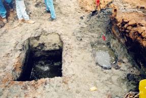 These
observations were made possible by digging a series of shallow trenches (Figure
85 and 86) and installation of some shallow (5 to 10 foot deep) 24-inch
diameter monitor wells (Figure 87). The trenches were dug to a depth of 36
inches and were then filled with water for gas bubble observations. They did
not penetrate the shallow ground water at 5 to 7 feet below surface in this
area. Measurement of the gas flux from a trench using a standard flux chamber
is shown in Figure 86.
These
observations were made possible by digging a series of shallow trenches (Figure
85 and 86) and installation of some shallow (5 to 10 foot deep) 24-inch
diameter monitor wells (Figure 87). The trenches were dug to a depth of 36
inches and were then filled with water for gas bubble observations. They did
not penetrate the shallow ground water at 5 to 7 feet below surface in this
area. Measurement of the gas flux from a trench using a standard flux chamber
is shown in Figure 86.
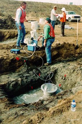 A 24-inch PVC
casing was installed and filled with coarse gravel, allowing gas flux to be observed
and measured at some of the most anomalous soil gas sites. In contrast to the
trenches, the 24-inch FW wells penetrated the shallow ground water table
adequately to allow observation of gas bubbles within the aquifer. This well
was often referred to as Mr. Bubble, but was not unique, since several of these
wells exhibited vigorous gas bubbling. Initial observations made before these
24-inch wells were cased indicated that the gases were entering more from the
sides than from the bottom, indicating that they did not intersect natural,
vertical migration pathways, and would, in all likelihood stop venting when the
shallow sands were depleted. They did, however, amply illustrate the
tremendous gas charging of the shallow subsurface within the areas containing
the larger methane concentrations.
A 24-inch PVC
casing was installed and filled with coarse gravel, allowing gas flux to be observed
and measured at some of the most anomalous soil gas sites. In contrast to the
trenches, the 24-inch FW wells penetrated the shallow ground water table
adequately to allow observation of gas bubbles within the aquifer. This well
was often referred to as Mr. Bubble, but was not unique, since several of these
wells exhibited vigorous gas bubbling. Initial observations made before these
24-inch wells were cased indicated that the gases were entering more from the
sides than from the bottom, indicating that they did not intersect natural,
vertical migration pathways, and would, in all likelihood stop venting when the
shallow sands were depleted. They did, however, amply illustrate the
tremendous gas charging of the shallow subsurface within the areas containing
the larger methane concentrations.
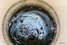 Data from
analyses of gas samples collected by volume displacement from the first two
trench wells, T-1 and T-2 contained 62.90% to 76.16% methane. These
concentrations are in the same general range as the soil gases collected from
four foot soil gas probes from this area. These trench samples were collected
by volume displacement, with the venting gases displacing the water in the
inverted bottles within seconds. Using a volume displacement gas collection
method ensured that the bottles contained 100% soil gas emitted directly from
the shallow sediments, with no air from the atmosphere during the sample
collection, yet air was found in the bottles. The presence of 23 to 36% air in
these samples implies that the air was part of the soil gas mixed with the
methane discharging from the shallow sands. The presence of air within such
shallow gas filled sediments would provide ideal conditions for oxidation of
the hydrocarbon gases in-situ.
Data from
analyses of gas samples collected by volume displacement from the first two
trench wells, T-1 and T-2 contained 62.90% to 76.16% methane. These
concentrations are in the same general range as the soil gases collected from
four foot soil gas probes from this area. These trench samples were collected
by volume displacement, with the venting gases displacing the water in the
inverted bottles within seconds. Using a volume displacement gas collection
method ensured that the bottles contained 100% soil gas emitted directly from
the shallow sediments, with no air from the atmosphere during the sample
collection, yet air was found in the bottles. The presence of 23 to 36% air in
these samples implies that the air was part of the soil gas mixed with the
methane discharging from the shallow sands. The presence of air within such
shallow gas filled sediments would provide ideal conditions for oxidation of
the hydrocarbon gases in-situ.
The methane isotopes for these two samples are nearly identical at –59.30 and –59.28 parts per thousand with respect to the PDB standard, and are comparable to the isotopic values noted within the 50-foot Ballona gravel monitor wells. Thus, the methane contained in the gravel aquifer does not appear to have been further oxidized within this very shallow sand. The carbon isotopic composition of ethane, on the other hand, yielded values of –17.94 to -13.62 parts per thousand with respect to the PDB standard. These are the heaviest values found on the site, out of over 80 individual analyses.
In contrast, the ethane in the 50-foot deep Ballona gravel aquifer monitor wells is much lighter, and has ethane carbon isotopic values that range from –18 to –21 parts per thousand. Although these aquifer isotope values are heavier than typical petroleum reservoir values, which normally range from about –29 to –32 parts per thousand, they are fairly consistent with other values measured in the aquifer, and definitely lighter than these two trench gas samples. Such heavy ethane isotope values in the trench samples would suggest biodegradation, either very near the surface, or somewhere along the migration pathway between the aquifer and the surface. Because of the large free gas discharge rates (liters per minute) from these two shallow trenches it would be unlikely for the observation of air in these samples to be a sampling artifact. This air must have naturally diffused into the shallow sediments where it mixed with the methane gas from depth, and was then discharged with the seepage gases when the surface cover was removed by digging and installing the trenches. It certainly seems impossible for soil gases bubbling directly out of the shallow sediments to contain 30% air, but there doesn’t appear to be any other reasonable explanation. The gas collected by volume displacement contained 62.90% to 76.16% methane.
Repeated soil gas sampling at different times within one of the macro-seepage areas north of Jefferson Avenue also provided some additional conformational variations that demonstrate how soil moisture changes can change the concentrations and degradation levels of the soil gas measured in a specific macro-seep. This macro-seepage area was initially sampled in 1998 when the ground was too wet for collection of a subsurface vapor sample. The crew observed bubbles venting into the atmosphere, and instead collected an atmospheric vapor sample over the bubbling seep. Although the sample was diluted with ambient air, it still contained a methane concentration of 0.4% which had a stable carbon isotopic value of –39.95 parts per thousand. This is a very mature carbon isotopic value which could possibly be generated by oxidation of the methane in the sample. Two other samples collected at about the same time had very appreciable methane and ethane soil gas concentrations. One contained 83.8% methane and 0.4% ethane, and another sample contained 41.2% methane and 0.3% ethane. These samples clearly contained gases that were not present in the atmosphere and demonstrated that methane and ethane were venting into the atmosphere.
In October/November of 1999, soil gas in this area was sampled at four feet (sites S77 and S78). No moisture problems were encountered and very large magnitude soil gas anomalies were found. The methane and ethane concentrations and their stable carbon isotopic values were as follows:
|
Site |
Methane |
Ethane |
Methane Δ13C |
Ethane Δ13C |
|
|
(%) |
(ppmv) |
(parts per mil) |
(parts per mil) |
|
S77 |
70.66 |
2400 |
-58.74 |
-20.57 |
|
S78 |
56.32 |
2900 |
-52.46 |
-19.92 |
These concentrations and isotopic values are comparable to those observed in the gravel aquifer monitor well MMW77 that underlies these soil gas anomalies. The measured values in the monitor well were:
|
Site |
Methane |
Ethane |
Methane Δ 13C |
Ethane Δ 13C |
|
|
(%) |
(ppmv) |
(parts per mil) |
(parts per mil) |
|
MMW77 |
89.02 |
3400 |
-59.95 |
-20.49 |
The larger soil gas sample (S77) is very similar in both composition and isotopic ratio to the dissolved gases in the gravel aquifer 50 feet below the surface, suggesting that at site S77 gas is venting from the aquifer with very little or no degradation. The CO2 soil gas values for these two samples are 5.56 and 16.65% respectively, indicating an increased level of degradation (oxidation) for S78 over S77. The very slight changes in the methane and ethane isotopes are consistent with minor biodegradation of the hydrocarbons and may be related to the larger quantity of CO2 measured at S78.
Nearly a year later (in August 2000) a second survey was conducted over this same area. On resurvey, values that had been as high as 75% now ranged only to 25% methane. The sites with the largest magnitude (sites 5011 and 5018) measurements are:
|
Site |
Methane |
Ethane |
Methane Δ 13C |
Ethane Δ 13C |
|
|
(%) |
(ppmv) |
(parts per mil) |
(parts per mil) |
|
5011 |
25.33 |
1100 |
-51.63 |
-16.83 |
|
5018 |
10.16 |
400 |
-45.09 |
-14.37 |
Although soil moisture was not measured, the sampling crew did believe that conditions were drier than before, and that reduced moisture had allowed more exchange with the atmosphere. This may have significantly affected the oxidation of both methane and ethane, particularly at site 5018, where the methane isotope had been increased to -45.09 and the ethane isotope had been increased to -14.37; values very close to what had been observed in a trench vent sample that was mixed with air. This example demonstrates that even a macro-seep site can change in direct response to changing surface conditions.
Special Considerations Regarding Soil Gas Carbon Dioxide
Most of this paper has dealt with establishing the nature and presence of natural hydrocarbon seepage and in defining some of the major controlling factors that must be accounted for in carrying out a near-surface soil gas investigation. There has been limited discussion of CO2 to this point although it has been measured in every Playa Vista sample. As we have mentioned earlier, carbon dioxide may be generated by the microbial oxidation of all types of organic materials, whether natural, or petroleum based (crude oil, gasoline, diesel, kerosene, chlorinated solvents, or just methane). For carbon sequestration monitoring it will be necessary to separate the biogenic CO2 from the injected CO2 that might have migrated from a reservoir.
The average concentration of carbon dioxide in ambient air, although increasing at noticeable rates, is only ~0.03 percent. Biodegradation of typical soil organic matter generally yields carbon dioxide concentrations between 0.2 and 5 percent. Higher concentrations of carbon dioxide measured in various soil vapor samples collected in the vicinity of subsurface petroleum contamination may yield values as high as 5 to 30 percent, an indication that biodegradation is significantly enhanced. Carbon dioxide concentrations in the Playa Vista data have this same range, with numerous soil gas CO2 anomalies in the range 20 to 30%. When the larger methane and CO2 maps are viewed on the regional scale, it is apparent that there is a spatial correlation between these two gases. The larger “biogenic CO2” anomalies always occur within the same general areas and in close proximity to the larger methane anomalies, but not necessarily at the same site. This lack of a point to point correlation is caused by the fact that the “biogenic CO2” did not migrate from the same deep source as the hydrocarbons, but instead is generatednear the seep where adequate oxygen is available. In addition, the “biogenic CO2” is only generated in fairly close proximity to its source (the seep), and then often in a “halo” pattern that places the largest concentrations of “biogenic CO2” close to, but not at the exact same physical location. If the seep is not too active, so that oxygen can infiltrate into the sampling point, then the “biogenic CO2” can be at the same site. The larger the seep becomes, then the more that the “biogenic CO2” may be displaced from the seep maximum, as shown by the example above in Figures 79, 80 and 81. This behavior has been documented by many environmental remediation surveys, such as the next two examples.
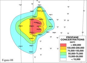
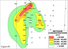
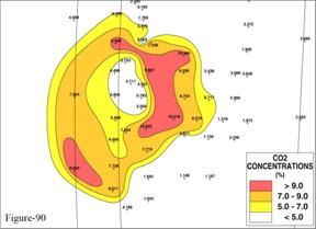
One of the most unique examples is shown by Figures 88, 89 and 90, taken from a detailed soil vapor survey conducted in Guadalajara, Mexico. This sampling grid consists of several infill samples collected on 5 to 10 meter spacing in the vicinity of a very large magnitude propane soil vapor anomaly that was discovered as part of a much larger regional survey. The ratio of propane to butanes and ethane indicated that the source of contamination was leakage of LNG (liquid natural gas) utilized throughout Mexico by residences and businesses. This propane anomaly was located in the garden area of a Social Services Building Complex. It is unusual to find a propane anomaly in the ground because the propane bottles are almost always mounted on the roofs. When this anomaly was discovered the local officials were unaware of any propane sources on the property. During excavation and gas monitoring operations, abandoned lines and valves were discovered in the garden area of the complex. A box containing corroded valves and distribution lines were found at the location containing the highest concentrations of propane. Unfortunately the supply lines were still connected to the sources on the roof and had begun to leak. The valves and lines were removed and a vapor extraction system was installed to vent the potentially explosive gases.
This propane anomaly shown in Figure 88 provides an excellent example where carbon dioxide (Figure 90) has likely been generated from oxidation of this “cookstove” propane in areas where oxygen is available either from oxygen or other anaerobic electron acceptors; and methane has been formed from its reduction (methanogenesis) in areas where methanogenic conditions develop. All of these processes occur within the influence of all types of near surface organic contamination, such as in this special case created by a propane leak. The highest methane and carbon dioxide concentrations can clearly form halos around the edges of the highest propane concentrations associated with the leaking propane fuel. Often, discussions concerning the biological generation of methane have focused on whether it is generated from the contaminant or from other, perhaps natural, organic matter. In this special case the local soils are made from volcanic tuff and are much too low in natural organic matter to serve as a source, so this appears to be a case where the propane fuel source is oxidized, either aerobically or anaerobically to carbon dioxide, followed by its reduction to methane.
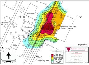
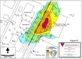
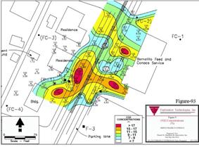
A second example, on Figure 91, shows the soil vapor analytical results and a contoured plume map for C5+ gasoline contamination. This plume indicated the presence of subsurface petroleum product contamination both on and off of the service station property. Extensive off-site migration of gasoline contamination was indicated beneath the major road located west of the station. All constituent plume maps were similar in areal extent and indicated that the source of the subsurface contamination was a release (or releases) of gasoline at the service station The methane and CO2 maps are shown in Figures 92 and 93, respectively. The methane plume is coincident with the gasoline and CO2 forms a “halo” around the gasoline contaminated area.
Surveys conducted over reservoirs selected for carbon sequestration should begin with a regional soil gas survey designed to locate seeps that are associated with the reservoir. Exploration examples integrated with available geological and geophysical data can provide initial guidance for these regional grids. These regional results will allow more focused infill surveys that can refine the locations of the most promising micro- and/or macro-seeps as possible locations for permanent monitoring stations. The Playa Vista example demonstrated the importance of sample spacing for precisely defining the actual locations of the seepage points where carbon sequestration flux monitoring stations should be located if they are to have a reasonable change of success. Because “biogenic CO2” is generated as a secondary product associated with the natural seeps, even more detailed surveys must be conducted in close proximity to these potential permanent monitoring stations in order to define any “biogenic CO2” associated with these specific hydrocarbon seeps. Experience gained conducting environmental surveys has demonstrated the stability of the hydrocarbon seeps and their associated “biogenic CO2”. Once determined they are very stable and can be used as a background against which any changes can be measured. Long term monitoring can be conducted by establishing a permanent monitoring station, or the soil gas survey can be rerun on a periodic basis.
The determination of the natural background of the methane through butane hydrocarbons and carbon dioxide is an exceedingly important task that must be completed before any locations are selected for monitoring CO2 in a carbon sequestration program. A review of the carbon sequestration literature has indicated that no soil gas surveys have been conducted in order to locate appropriate sites for flux stations, and that all of the monitoring stations have been randomly placed. The monitoring focus has been placed on setting up flux chambers and vertically nested monitoring wells, without any guidance from a gridded soil gas data set (Klusman, 2003, 2005, Nance, 2005). As pointed out in the introduction in this paper, we believe that addition of tracers is not initially required, particularly when injecting CO2 into old oil and/or gas fields. Hydrocarbons reservoirs contain their own tracers, in the form of ethane, propane and butanes, which are present in all petroleum reservoirs. Tracers can be usefully employed after successful flux measurements have been accomplished when there is the need to determine residence and migration transit times.
The limited carbon sequestration related monitoring to date appears to have been done with the assumption that the earth is isotropic and homogeneous. Nothing could be farther from the truth. Natural seepage everywhere on the surface of the earth is distributed in “localized gas anomalies” that form dendritic patterns that look much like the examples shown in this paper. The planning for monitoring CO2 leakage associated with carbon sequestration projects requires separating the injected CO2 from the “biogenic CO2” and/or the natural CO2 present in the near-surface soils before the project is initiated. Once these latter two CO2 distributions are known, then the injected CO2 can easily be recognized because it will change these natural patterns. The analytical protocols and data validation that have been employed for carbon sequestration related monitoring to date appear excellent provided that they are placed in the proper locations.
Agostino, P.N., Jones V.T., and Le Blanc, Jr., R., 1999, Assessment and Remediation of Hydrocarbon Contamination in a Latin American Petroleum Facility, Presented at the AAPG Annual Convention, April 11-14, San Antonio, TX.
Barsukov, V.L., 1979, Geochemical methods of predicting earthquakes: Geochemistry International, V. 16, No. 2, pp. 1-13.
Bray, M. and Jones, V.T., 1985. Correlation of Spacial and Compositional Discriminators of North American Hydrocarbon Basins. American Chemical Society, Chicago, ILL, September 10.
Borodzich, E.V., 1979, Preliminary results on helium pattern variations in seismically active zones: Geochemistry International, V. 16, No. 2, pp. 37-41.
Burtell, S.G., Jones V.T., and Anderson, T.A., 1987. Spatial Relationships Between Macroseeps From A Thermal Spring and Free Soil Gases Measured by Shallow 4 Foot Probe. Presented at Fifth Thematic Conference, Reno, NV.
Burtell, S. G., 1989, Geochemical investigations at Arrowhead Springs, San Bernardino and along the San Andreas Fault in Southern California: MS Thesis, University of Pittsburgh.
Craig, H., Chung, Y., Lupton, J.E., Damasceno, S., Poreda, R., 1980, Investigation of radon and helium as possible fluid phase precursors to earthquakes: Technical Report 13, United States Geologic Survey Contract #USGS 14-08-0001-18348, 36 pages.
Drozd, R.J., Pazdersky, G.J., Jones, V.T., and Weismann, T.J., 1981, Use of compositional indicators in prediction of petroleum production potential (abs.). Presented at: the 1981 American Chemical Society Meeting, Atlanta, GA., March 29-April 3.
Elinson, M.M., Pashkov, Y.N., Agababov, G.M., and Ignatiev, I.B., 1970, Measurements of gases distributed above Cu-Mo ore bodies. In: The Geochemistry of Hg, Mo and S in Hydrothermal Processes. Ed. Nauka, Moscow.
Eremeev, A.N., Sokolov, V.A., and Yanitskii, I.N., 1973, Applications of helium surveying to structural mapping and ore deposit forecasting. In: M.J. Jones (Editor), Geochemical Exploration 1972. Institution of Mining and Metallurgy, London, pp. 177-183.
Fursov, V.Z., Vol'fson, and Khvalorski, A.G. 1968, Results of a study of mercury vapor in the Tashkent Earthquake Zone: Dolk Acad. Navk USSR, Vol 179, No. 5, pp. 1213-1215.
Gunter, B.D., 1978, C1-C4 hydrocarbons in hydrothermal gasses: Geochemica et Cosmochimica Acta, Vol. 42, pp. 137-139.
Hadley, D. and Kanamori, H., 1977, Seismic structures of the Transverse Ranges, California: Geologic Society of America Bull., V. 88, p. 1469-1478.
Hirst, W., Gibson, G., Gillespie, S., Archibald, I., Podlaha, O., Skeldon, K., Courtrial, J., Monk, S. and Padgett, M., , 2004, Oil and gas prospecting by ultra-sensitive optical gas detection with inverse gas dispersion modeling, GEOPHYSICAL RESEARCH LETTERS, VOL. 31, L12115, doi:10.1029/2004GL019678, 2004
Hunt, J.H., 1981, Surface geochemical prospecting pro or con. Invited Paper at: the AAPG Annual Convention, San Francisco, May. Hunt, J.M., 1979, Petroleum geochemistry and geology. W.H. Freeman, San Francisco, 617 pp.
Iacopi, Robert, 1976, Earthquake Country, Lane Books, Menlo Park, California, p. 87.
Jones, V.T., and Drozd, R.J., 1976, Predictions of oil and gas potential by near-surface geochemistry: AAPG Annual Meeting, Abstract only, Bull., Vol. 63, p. 699.
Jones V.T., and Sidle, W.C., 1982. Light Hydrocarbon, Hydrogen and Helium Anomalies in the Eastern Snake River Plain. Paper presented at ACS Meeting, Los Vegas, Nevada.
Jones V.T., and Burtell, S.B., 1983. Gas Monitoring at Arrowhead Hot Spring Near the San Andreas Fault, San Bernardino County, California. American Chemical Society Meeting, Washington, DC, August.
Jones, V.T., 1983. Surface Monitoring of Retort Gases from an Underground Coal Gasification Reactor: Time Dynamics. American Chemical Society, Washington, DC, August.
Jones, V.T., 1984. Overview of Hydrocarbon Extractions in Soil and Waters: Research Needs and Problems. Presented at API Workshop for Sampling and Analytical Methods for Determining Petroleum Hydrocarbons in Groundwater ands Soil, Denver.
Jones, V.T. and Bray, M., 1985. Compositional Correlations Between Subsurface Wells and Surface and Marine Geochemical Data. American Chemical Society Meeting, Miami Beach, FL, April 30-May 1.
Jones, V.T., Burtell, S.G, Hodgson, R.A., Whelan, T., Milan, C., Ando, T., Okada, K., Agatsuma, T,. Takano, O., 1985. Remote Sensing and Surface Geochemical Study of Railroad Valley, Nye County, Nevada. Proceedings of the International Symposium Remote Sensing of Environment, Fourth Thematic Conference, Remote Sensing for Exploration Geology, April 1-4, pp. 381-389.
Jones, V.T, 1987. Review of Onshore Hydrocarbon Seepage. Presented at the Research Conference on Vertical Hydrocarbon Migration: Geological, Geochemical, and Geophysical Expressions, Session II, Geochemical Aspects of Vertical Hydrocarbon Migration, Institute for the Study of Earth and Man at SMU, Ft. Burgwin Research Center, Taos, N.M., October 15-19.
Jones, V.T, 1987. Flux Rates of Vertical Migration - Chromatographic Effects and Time Dynamics. Presented at the Research Conference on Vertical Hydrocarbon Migration: Geological, Geochemical, and Geophysical Expressions, Session II, Geochemical Aspects of Vertical Hydrocarbon Migration, Institute for the Study of Earth and Man at SMU, Ft. Burgwin Research Center, Taos, N.M., October 15-19.
Jones, V.T, 1987. Seismic Velocity Changes in Geochemical Leakage Chimneys: Documentation of Surface Geochemical Anomalies with Zones of Seismic Disturbance. Presented at the Research Conference on Vertical Hydrocarbon Migration: Geological, Geochemical, and Geophysical Expressions, Section VI, Electrical and Other Geophysical Aspects of Vertical Hydrocarbon Migration, Institute for the Study of Earth and Man at SMU, Ft. Burgwin Research Center, Taos, N.M., October 15-19.
Jones, V.T, 1994, Soil Gas Calibration Surveys Over the Filo Morado and Loma de La Lata Oil & Gas Fields in the Neuquen Basin, Argentina. Presented AAPG Hedberg Research Conference, Near-Surface Expression of Hydrocarbon Migration, Vancouver, British Columbia, Canada,(Abstract, Special Print) April 24-28, 1994.
Jones, V.T, S.G. Burtell, and D.A. Link, 1996, Surface Geochemical Applications to Petroleum Exploration. Presented at the 5th Latin American Congress on Organic Geochemistry, October 6-10, 1996, Cancun, Mexico.
Jones, V.T, 1997, Innovative Screening Technologies Allow Cost-Effective Accelerated Site Assessments, Presented at the Houston Geological Society, February 12, 1997, Houston, TX.
Jones, V.T, and S.G. Burtell, 1998, Surface Geochemical Applications to Petroleum Exploration. Presented at the 215th American Chemical Society National Meeting and Exposition, April, 1998, Dallas, TX.
Jones, V.T, 1998, Applications of Soil Gas Geochemical Methods in the Detection and Mapping of Underground Contamination, Presented at the Texas Association of Environmental Professionals Meeting, Sept. 1998, Houston, TX.
Jones, V.T and Agostino, P.N., 1999, Surface Geochemical Applications to Petroleum Exploration, Presented at the AAPG Annual Convention, April 11-14, 1999, San Antonio, TX.
Jones, V.T, 2000a, Application of Forensic Geochemical Methods in Assessment of Hydrocarbon Release, Presented at the Energy and the Environment: Challenges of the Future Symposium; University of Pittsburgh, Department of Geology and Planetary Sciences, April 7, Pittsburgh, PA.
Jones, V.T, 2000b, Surface Geochemical Applications to Petroleum Exploration, Presented at the Energy and the Environment: Challenges of the Future Symposium, University of Pittsburgh, Department of Geology and Planetary Sciences, April 8, Pittsburgh, PA.
Jones, V.T., Coleman, D.D., Becker, D.F., Anderson, T.H., Witherspoon, P.A., Robbins, G.A., 2002: Surface and Near-Subsurface Hydrocarbon Migration Patterns Associated with a Macroseep. AAPG: Successful Application of Non-Seismic Techniques to Exploration, AAPG Annual Convention, Houston, TX.
(an AAPG Talk of the unfinished Playa Vista Report - July 10,2001)
Kartsev, A.A., Tabarsaranskii, Z.A., Subbota, M.I., and Mogilevskii, G.A., 1959, Geochemical methods of prospecting and exploration for petroleum and natural gas: University of California Press, Berkeley, 349 pp.
King, Chi-Yu, 1980, Geochemical measurements pertinent to earthquake prediction: J. Geophy. Res., V. 85, No. 136, June 10, 3051 pp.
Klusman, R. W., 2003, A Geochemical Prospective and Assessment of Leakage. Potential for a Mature Carbon Dioxide EOR Project, and as a Prototype for Carbon Dioxide Sequestration; Rangely Field Colorado, USA, AAPG Bull., 87, pp. 1485-1507.
LeBlanc, Jr., R.J., and V.T.Jones, 2004b, Criteria for a multi-disciplined approach for exploration, exploitation, and development drilling in the Morrow incised-valley oil trend of Colorado and Kansas: The 3-G method, Abstract, Rocky Mountain Section AAPG Meeting, August 9-11, 2004, Denver, Colorado.
Mamyrin, B.S., 1979, 3He/4He Ratios in earthquake forecasting: Geochemistry International, V. 16, No. 2, pp. 42-44.
McNerney and Buseck, 1973, Economic Geology, Q8, 1313 -1320.
McCurdy, R., 1979, Site qualification studies of the UCG-SDB site, North Knobs, Wyoming. Prepared by GS&T under DOE contract De-AC03-77-ET13108, May 23. C&M Division Report 64RK076.
Melvin, J.D., Shapiro, M.H., and Copping, N.A., 1978, An automated radon-thoron monitor for earthquake prediction research: Nucl. Instrum. and Methods, 153, pp. 239-251.
Miller, K.F., 1979, Geologic map of the San Bernardino North Quadrangle, California: Department of Interior, United States Geologic Survey Open File Report 79-770.
Mooney, J.R., 1982, Sniffing for oil and earthquakes: The Orange Disk, V. 25, No. 9, pp. 26-29.
Mousseau, R.J. and J.C. Williams, 1979, Dissolved hydrocarbons in coastal waters of North America (abs.): A.A.P.G. Bulletin, v. 63, p. 699-700.
Mousseau, R.J., 1980, Marine hydrocarbon prospecting geochemistry: Proceedings of the Ninth Annual Meeting, Indonesian Petroleum Association, Jakarta, Indonesia. May.
Mousseau, R.J., and W.H. Glezen, 1980, The Gulf marine hydrocarbon sampling and analysis system: Proceedings of a Symposium and Workshop on Water Sampling while Underway, National Academy Press, Washington D.C., Feb. 11-12, p. 167- 192.
Mousseau, R.J., 1981a, Role of R/V Hollis Hedberg in marine hydrocarbon geochemical prospecting on continental margins: S.W. Sec. Soc. of Exploration Geophysicists, New Orleans, LA., February.
Mousseau, R.J., 1981b, Role of R/V Hollis Hedberg in marine hydrocarbon geochemical prospecting on continental margins: AAPG Hedberg Research Conference on Continental Margin Processes, Galveston, Texas, January.
Mousseau, R.J., 1983, Underway sampling and analysis of oceanic hydrocarbons for petroleum exploration: American Chem. Soc. National Meeting, Atlanta, GA. March.
Nance, H. S., Rauch, Henry, Brian Strazisar, Grant Bromhal, Art Wells, Rod Diehl, Ron Klusman, Jennifer Lewicki, Curt Oldenburg, Yousif K. Kharaka, Evangelos Kakouros, 2005, Surface Environmental Monitoring At the Frio CO2 Sequestration Test Site, Texas, 4th Annual Conference on Carbon Capture and Sequestration Alexandria, Virginia May 2–5.
Ovchinnikov, L.N., Sokolov, V.A., Fridman, A.I., and Yanitskii, I.N., 1972, Gaseous geochemical methods in structural mapping and prospecting for ore deposits. In: M.J. Jones (Editor), Geochemical Exploration, 1972. Institution of Mining and Metallurgy, London, pp. 177-183.
Pirkle, R.J., 1985, Hydrocarbon seeps in the Gulf of Mexico. Presented at: the 189th ACS National Meeting American Chemical Society, Miami Beach, Florida. April 28-May 3, paper no. 78.
Pirkle, Robert J., 1986, Near Surface Geochemical Monitoring of Underground Gas Storage Facilities, Presented at: The American Gas Association Meeting, Chicago, IL, April.
Pirkle, R. J. and Price, Van, 1986, Leak Detection and Monitoring, Paper presented at: The Conference on Hazardous Materials in the Environment, Atlantic City, NJ, June.
Pirkle, Robert J., Wyatt, Douglass E., Price, Van, and Looney, Brian B., 1992, Barometric Pumping: The Connection Between the Vadose Zone and the Atmosphere, Presented at: The Focus Eastern Regional Groundwater Issues Conference, Newton, MA., October.
Preston, Don, 1980, Gas eruptions taper off in northwest Oklahoma: Geotimes, October, pp 18-26.
Pruess, Karsten, Barry Freifeld, Mack Kennedy, Curt Oldenburg, Tommy J. Phelps, M.C. van Soest, Use of Gas Phase Tracers for Monitoring CO2 Injection at the Frio Test Site, 4th Annual Conference on Carbon Capture and Sequestration Alexandria, Virginia, May 2–5.
Reimer, D.M., 1980, Use of soil gas helium concentrations for earthquake prediction, limitations imposed by diagonal variation: J. Geophy. Res., V. 85, No. 136, June 10, pp. 3107-3114.
Richers, D.M., 1984, Comparison of commonly applied soil-gas techniques used in evaluating hydrocarbon potential. Presented at 187th Annual Meeting, American Chemical Society, St. Louis, MO, April.
Richers, D.M., Jones, V.T., Matthews, M.D., Maciolek, J.B., Pirkle, R.J., and Sidle, W.C., 1986. A Landsat - Soil Gas Geochemical Survey of the Patrick Draw Area, Sweetwater County, Wyoming, 1983-Survey. AAPG Bulletin, Vol. 70, No. 7.
Shapiro, M.H., Melvin, J.D., Tombrello, T.A., Mendenhall, M. H., Larson, P.B., and Whitcomb, J.H., 1981, Relationship of the 1979 Southern California radon anomaly to a possible regional strain event: J. Geophys. Res., V. 86, 1725 pp.
Sokolov, V.A., 1971, Geochemistry of natural gases: Niedra, Moscow. Southern Sierra Power Company, 1925, Geothermal areas adjacent to the transmission lines of the Southern Sierra Power Company, Geothermal Resource Council Special Report #3, Geothermal Exploration in the First Quarter Century, pages 145-161.
Wakita, H., 1978, Helium spots: caused by diapiric magma from the Upper Mantle: Science, V. 200, April 28, pp. 430-432.
Zorkin, L.M., Zabairaevi, S.L., Karus, E.V., Kilmetov, K. Kh., 1977, Experience of geochemical prospecting in petroleum and gas deposits in the seismically active zone of Sakhalin Island, IZU (Russ.). UZSSh Uchebn. Zaved, Geol. Razved, V. 20, pp. 52-62.
HTML
Austin Tankfarm - http://eti-geochemistry.com/aapg48/index.html
Case Studies of Anaerobic Methane - http://eti-geochemistry.com/anaerobic/index.html
Coal Bed Methane - http://eti-geochemistry.com/jonesandthune/index.html
Elsevier - Handbook of Exploration Geochemistry: Geochemical Remote Sensing of the Sub-Surface - http://eti-geochemistry.com/elsevier/index.html
Filo Mirado - http://eti-geochemistry.com/neuquen/index.html
Forensic Geochemistry - http://eti-geochemistry.com/forensic/index.html
Hedberg Rules! - Gulf Science & Technology Company - (Gulf Oilmanac 6-80, pp. 2-4) - http://eti-geochemistry.com/oilmanac680/index.html
Helium/Hydrogen - http://eti-geochemistry.com/helium/index.html
High Island - http://eti-geochemistry.com/highisla/index.html
Hydrocarbon Flux Variations in Natural & Manmade Seeps - http://eti-geochemistry.com/flux/index.html
Playa Vista Report - (April 2000) - /Report-04-2000/index.html
Playa Vista Report - (Regional) - /Regional/index.html
Predictions of Oil & Gas Potential by Near-surface Geochemistry: AAPG Annual Meeting - http://eti-geochemistry.com/j&d.html
"The Orange Disc", a Gulf Oil Magazine, Fall of 1982 - http://eti-geochemistry.com/gulfeq/index.html
Microsoft Power Point
Adsorbed Gas Talk - (Microsoft Power Point) - AAPG-adsorbed.ppt
Casing Leaks - (Microsoft Power Point) - Assessment of Casing Leaks VT Jones.ppt
Adobe Acrobat
Kansas: A Successful Integration of Surface Soil Gas Geochemistry with Geology & Geophysics - Kansas-RMAG-paper-rev3.pdf
Lost River Paper - AAPG Abstract 2006 - (Abode Acrobat) - LostRiverAAPG2006abstract.pdf
How to Design an Exploration Surface Soil Gas Geochemical Survey - Howto04.pdf